Slope Stability.pdf
This document was uploaded by user and they confirmed that they have the permission to share it. If you are author or own the copyright of this book, please report to us by using this DMCA report form. Report DMCA
Overview
Download & View Slope Stability.pdf as PDF for free.
More details
- Words: 6,559
- Pages: 41
Loading documents preview...
Slope Stability Thursday, March 11, 2010 11:43 AM
Slope and excavation stability analyses are used in a wide variety of geotechnical engineering problems, including, but not limited to, the following: • Determination of stable cut and fill slopes
• Assessment of overall stability of retaining walls, including global and compound stability (includes permanent systems and temporary shoring systems) • Assessment of overall stability of shallow and deep foundations for structures located on slopes or over potentially unstable soils, including the determination of lateral forces applied to foundations and walls due to potentially unstable slopes
• Stability assessment of landslides (mechanisms of failure, and determination of design properties through back-analysis), and design of mitigation techniques to improve stability • Evaluation of instability due to liquefaction
(From WASDOT manual of instruction)
Steven F. Bartlett, 2010
Slope Stability Page 1
Types of Mass Movement (i.e., Landsliding) Thursday, March 11, 2010 11:43 AM
General Types of Mass Movement
Morphology of a Typical Soil Slump Steven F. Bartlett, 2010
Slope Stability Page 2
Required Soil Parameters Thursday, March 11, 2010 11:43 AM
Whether long-term or short-term stability is in view, and which will control the stability of the slope, will affect the selection of soil and rock shear strength parameters used as input in the analysis. For short-term stability analysis, undrained shear strength parameters should be obtained. Short-term conditions apply for rapid loadings and for cases where construction is completed rapidly (e.g. rapid raise of embankments, cutting of slopes, etc.) For long-term stability analysis, drained shear strength parameters should be obtained. Long-term conditions imply that the pore pressure due to the loading have dissipated and the equilibrium pore pressures have been reached.
For assessing the stability of landslides, residual shear strength parameters will be needed, since the soil has in such has typically deformed enough to reach a residual value. This implies that the slope or soil has previously failed along a failure plane and the there is potential for reactivation of the failure along this plane. For highly overconsolidated clays, such as the Seattle clays (e.g., Lawton Formation), if the slope is relatively free to deform after the cut is made or is otherwise unloaded, residual shear strength parameters should be obtained and used for the stability analysis.
Steven F. Bartlett, 2010
Slope Stability Page 3
Factors of Safety for Slopes and Embankments Thursday, March 11, 2010 11:43 AM
Factors of safety for slopes other than the slopes of dams should be selected consistent with the uncertainty involved in the parameters such as shear strength and pore water pressures that affect the calculated value of factor of safety and the consequences of failure. When the uncertainty and the consequences of failure are both small, it is acceptable to use small factors of safety, on the order of 1.3 or even smaller in some circumstances. When the uncertainties or the consequences of failure increase, larger factors of safety are necessary. Large uncertainties coupled with large consequences of failure represent an unacceptable condition, no matter what the calculated value of the factor of safety.
The values of factor of safety listed in Table 3-1 provide guidance but are not prescribed for slopes other than the slopes of new embankment dams. Typical minimum acceptable values of factor of safety are about 1.3 for end of construction and multistage loading, 1.5 for normal long-term loading conditions, and 1.1 to 1.3 for rapid drawdown in cases where rapid drawdown represents an infrequent loading condition. In cases where rapid drawdown represents a frequent loading condition, as in pumped storage projects, the factor of safety should be higher. (from US Army Corp EM 1110-2-1902) Reliability analysis techniques can be used to provide additional insight into appropriate factors of safety and the necessity for remediation. (from US Army Corp EM 1110-2-1902)
Note that for long-term stability of natural or cut slopes, a factor of safety of 1.5 is usually selected for cases where failure of the slope could affect safety or property.
Steven F. Bartlett, 2010
Slope Stability Page 4
Analysis Methods - Limit Equilibrium Thursday, March 11, 2010 11:43 AM
Limit Equilibrium ○ Most common LE method is the method of slices ○ Methods/Researchers Ordinary Method of Slices Modified or Simplified Bishop Taylor Spencer Spencer-Wright Janbu Fellenius (Swedish) Morgenstern Morgenstern-Price US Army Corp of Engineers Bell Sharma General Limit Equilibrium Methods (GLE)
Steven F. Bartlett, 2010
Slope Stability Page 5
LE Analysis Methods - References Thursday, March 11, 2010 11:43 AM
Steven F. Bartlett, 2010
Slope Stability Page 6
Simplified Bishops Method Thursday, March 11, 2010 11:43 AM
Simplified Bishop's Method (from US Army Corp EM 1110-2-1902) a. Assumptions. The Simplified Bishop Method was developed by Bishop (1955). This procedure is based on the assumption that the interslice forces are horizontal, as shown in Figure C-11. A circular slip surface is also assumed in the Simplified Bishop Method. Forces are summed in the vertical direction. The resulting equilibrium equation is combined with the Mohr-Coulomb equation and the definition of the factor of safety to determine the forces on the base of the slice. Finally, moments are summed about the center of the circular slip surface to obtain the following expression for the factor of safety:
Steven F. Bartlett, 2010
Slope Stability Page 7
Simplified Bishops Method Example Thursday, March 11, 2010 11:43 AM
(from US Army Corp EM 1110-2-1902)
Steven F. Bartlett, 2010
Slope Stability Page 8
Simplified Bishops Method - Misc. Thursday, March 11, 2010 11:43 AM
Limitations. Horizontal equilibrium of forces is not satisfied by the Simplified Bishop Method. Because horizontal force equilibrium is not completely satisfied, the suitability of the Simplified Bishop Method for pseudo-static earthquake analyses where an additional horizontal force is applied is questionable. The method is also restricted to analyses with circular shear surfaces.
Recommendation for use. It has been shown by a number of investigators that the factors of safety calculated by the Simplified Bishop Method compare well with factors of safety calculated using more rigorous equilibrium methods, usually within 5 percent. Furthermore, the procedure is relatively simple compared to more rigorous solutions, computer solutions execute rapidly, and hand calculations are not very time-consuming. The method is widely used throughout the world, and thus, a strong record of experience with the method exists. The Simplified Bishop Method is an acceptable method of calculating factors of safety for circular slip surfaces. It is recommended that, where major structures are designed using the Simplified Bishop Method, the final design should be checked using Spencer’s Method. Verification procedures. When the Simplified Bishop Method is used for computer calculations, results can be verified by hand calculations using a calculator or a spreadsheet program, or using slope stability charts. An approximate check of calculations can also be performed using the Ordinary Method of Slices, although the OMS will usually give a lower value for the factor of safety, especially if φ is greater than zero and pore pressures are high.
Steven F. Bartlett, 2010
Slope Stability Page 9
Numerical Methods Thursday, March 11, 2010 11:43 AM
51st Rankine Lecture Geotechnical Stability Analysis Professor Scott W Sloan University of Newcastle,NSW, Australia ABSTRACT Historically, geotechnical stability analysis has been performed by a variety of approximate methods that are based on the notion of limit equilibrium. Although they appeal to engineering intuition, these techniques have a number of major disadvantages, not the least of which is the need to presuppose an appropriate failure mechanism in advance. This feature can lead to inaccurate predictions of the true failure load, especially for cases involving layered materials, complex loading, or three-dimensional deformation. This lecture will describe recent advances in stability analysis which avoid these shortcomings. Attention will be focused on new methods which combine the limit theorems of classical plasticity with finite elements to give rigorous upper and lower bounds on the failure load. These methods, known as finite element limit analysis, do not require assumptions to be made about the mode of failure, and use only simple strength parameters that are familiar to geotechnical engineers. The bounding properties of the solutions are invaluable in practice, and enable accurate solutions to be obtained through the use of an exact error estimate and automatic adaptive meshing procedures. The methods are extremely general and can deal with layered soil profiles, anisotropic strength characteristics, fissured soils, discontinuities, complicated boundary conditions, and complex loading in both two and three dimensions. Following a brief outline of the new techniques, stability solutions for a number of practical problems will be given including foundations, anchors, slopes, excavations, and tunnels.
Steven F. Bartlett, 2010
Slope Stability Page 10
Numerical Methods Thursday, March 11, 2010 11:43 AM
Numerical Modeling (FDM and FEM) Numerical model such as FLAC offers these advantages over Limit Equilibrium methods: • Any failure mode develops naturally; there is no need to specify a range of trial surfaces in advance. • No artificial parameters (e.g., functions for inter-slice angles) need to be given as input. • Multiple failure surfaces (or complex internal yielding) evolve naturally, if the conditions give rise to them. • Structural interaction (e.g., rock bolt, soil nail or geogrid) is modeled realistically as fully coupled deforming elements, not simply as equivalent forces. • Solution consists of mechanisms that are feasible kinematically. Pasted from
There are a number of methods that could have been employed to determine the factor of safety using FLAC. The FLAC shear strength reduction (SSR) method of computing a factor of safety performs a series of computations to bracket the range of possible factors of safety. During SSR, the program lowers the strength (angle) of the soil and computes the maximum unbalanced force to determine if the slope is moving. If the force unbalance exceeds a certain value, the strength is increased and the original stresses returned to the initial value and the deformation analyses recomputed. This process continues until the force unbalance is representative of the initial movement of the slope and the angle for this condition is compared to the angle available for the soil to compute the factor of safety. Steven F. Bartlett, 2010
Slope Stability Page 11
FLAC modeling - Total Stress vs. Effective Stress Analysis Thursday, March 11, 2010 11:43 AM
Short-term analysis (Immediate or sudden changes in load) ○ Effective stress analysis (drained parameters) (if pore pressure due to loading can be estimated, howeever often difficult to do this) ○ Total stress analysis (undrained parameters) (if pore pressure are not estimated and not present in the model)
Long-term analysis (pore pressure from change in loading have dissipated) ○ Effective stress analysis In FLAC, the yield criterion for problems involving plasticity is expressed in terms of effective stresses. The strength parameters used for input in a fully coupled mechanical-fluid flow problem are drained properties. Also, whenever CONFIG gw is selected: a) the drained bulk modulus of the material should be used if the fluid bulk modulus is specified; and b) the dry mass density of the material should be specified when the fluid density is given. The apparent volumetric and strength properties of the medium will then evolve with time, because they depend on the pore pressure generated during loading and dissipated during drainage. The dependence of apparent properties on the rate of application of load and drainage is automatically reflected in a coupled calculation, even when constant input properties are specified. Steven F. Bartlett, 2010
Slope Stability Page 12
FLAC modeling - Effective Stress Analysis Thursday, March 11, 2010 11:43 AM
Initializing Stress and Pore Pressures for Horizontally Layered Systems
config gw ex=4 g 10 10 mo e pro bulk 3e8 she 1e8 den 2000 por .4 pro den 2300 por .3 j 3 5 pro den 2500 por .2 j 1 2 pro perm 1e-9 mo null i=1,3 j=8,10 water bulk 2e9 den 1000 set g=9.8 call iniv.fis; this file must be present in project file folder set k0=0.7 i_stress fix x i 1 fix x i 11 fix y j 1 hist unbal set flow off step 1 save iniv.sav solve ret FLAC save initiate.sav 'last project state'
Steven F. Bartlett, 2010
Slope Stability Page 13
FLAC modeling - Effective Stress Analysis Thursday, March 11, 2010 11:43 AM
Initializing Stress and Pore Pressures for Horizontally Layered Systems JOB TITLE : .
(*10^1)
FLAC/SLOPE (Version 5.00) 1.000
LEGEND 30-Nov-10 18:26
0.800
Grid plot 0
2E 0
Pore pressure contours 0.00E+00 2.00E+04 4.00E+04 6.00E+04 8.00E+04 1.00E+05
0.600
0.400
Contour interval= 2.00E+04 0.200
0.000
Steven Bartlett University of Utah 0.000
0.200
0.400
0.600
0.800
1.000
(*10^1)
JOB TITLE : .
(*10^1)
FLAC/SLOPE (Version 5.00) 1.000
LEGEND 30-Nov-10 18:26
0.800
Grid plot 0
2E 0
Effec. SYY-Stress Contours -1.25E+05 -1.00E+05 -7.50E+04 -5.00E+04 -2.50E+04 0.00E+00
0.600
0.400
Contour interval= 2.50E+04 0.200
0.000
Steven Bartlett University of Utah 0.000
0.200
0.400
0.600 (*10^1)
Steven F. Bartlett, 2010
Slope Stability Page 14
0.800
1.000
FLAC modeling - Interface Considerations Thursday, March 11, 2010 11:43 AM
If a model containing interfaces is configured for groundwater flow, effective stresses (for the purposes of slip conditions) will be initialized along the interfaces (i.e., the presence of pore pressures will be accounted for within the interface stresses when stresses are initialized in the grid). To correctly account for pore pressures, CONFIG gw must be specified. For example, the WATER table command (in non-CONFIG gw mode) will not include pore pressures along the interface, because pore pressures are not defined at gridpoints for interpolation to interface nodes for this mode. Note that flow takes place, without resistance, from one surface to the other surface of an interface, if they are in contact. Flow along an interface (e.g., fracture flow) is not computed, and the mechanical effect of changing fluid pressure in an interface is not modeled. If the interface pore pressure is greater than the total stress acting across the interface (i.e., if the effective stress tends to be tensile), then the effective stress is set to zero for the purpose of calculating slip conditions.
Steven F. Bartlett, 2010
Slope Stability Page 15
FLAC Modeling - Total Stress Analysis Thursday, March 11, 2010 11:43 AM
For clayey material, the time required for dissipation of excess pore pressures developed by application of the load may be so long that undrained conditions may exist not only during, but for a long time after, loading. In this time scale, the influence of fluid flow on the system response may be neglected; if the fluid is stiff compared to the clay material (Kw >>> K + (4/3)G, where K and G are drained moduli), the generation of pore pressures under volumetric strain may strongly influence the soil behavior. In this situation, an undrained analysis can be applied. If the primary emphasis is on the determination of failure, and assuming a Mohr-Coulomb material with no dilation, two modeling approaches may be adopted in FLAC: 1. WET SIMULATION - The groundwater configuration (CONFIG gw) is adopted with a no-flow condition. Dry density, drained bulk and shear elastic moduli, and drained cohesion and friction angle are used in the input. In this approach effective stress strength properties are used because pore pressures are initialized in the model and the increase in pore pressure for the applied load is calculated by the model. Because pore pressures are present, then effective stress are appropriate and calculated for the undrained loading.) 2. DRY SIMULATION - The slope or foundation soil may be analyzed without taking the fluid explicitly into account. For this approach, total unit weight and undrained strength properties should be used throughout the model. For this simulation, the fluid is not explicitly taken into consideration, but its effect on the stresses is accounted for by assigning the medium an undrained bulk modulus. The groundwater configuration is not selected in this simulation, and a wet density ρu must be assigned to the saturated medium. In the following example, we make use of the material undrained shear strength; it is applicable if the following conditions hold: 1) plane-strain condition; 2) undrained condition; 3) undrained Poisson’s ratio νu is equal to 0.5; and 4) Skempton's pore pressure coefficient B is equal to one.
Steven F. Bartlett, 2010
Slope Stability Page 16
FLAC Modeling - Dry Simulation Thursday, March 11, 2010 11:43 AM
So that a dry simulation will yield comparable results to a wet simulation, the undrained cohesion must be calculated so that it is comparable to the drained friction angle, drained cohesion at the appropriate stress level (i.e., initial mean effective stress.) Because mean effective stress varies with depth, this means that the undrained cohesion must also vary with depth. This describes how this is done in FLAC and the limitations of a dry simulation.
Steven F. Bartlett, 2010
Slope Stability Page 17
Undrained Analysis - Wet Simulation Thursday, March 11, 2010 11:43 AM
; WET SIMULATION **** config gw ex 5 grid 20 10 model mohr def prop_val w_bu = 2e9 ; water bulk modulus d_po = 0.5 ; porosity d_bu = 2e6 ; drained bulk modulus d_sh = 1e6 ; shear modulus d_de = 1500 ; dry density w_de = 1000 ; water density b_mo = w_bu / d_po ; Biot modulus, M d_fr = 25.0 ; friction d_co = 5e3 ; cohesion end prop_val ; ini x mul 2 prop dens=d_de sh=d_sh bu=d_bu; drained properties prop poros=d_po fric=d_fr coh=d_co tens 1e20 water dens=w_de bulk=w_bu tens=1e30 set grav=10 ; --- boundary conditions --fix x i=1 fix x i=21 fix x y j=1 ; --- initial conditions --ini syy -2e5 var 0 2e5 ini sxx -1.5e5 var 0 1.5e5 ini szz -1.5e5 var 0 1.5e5 ini pp 1e5 var 0 -1e5 set flow=off ; ; --- surcharge from embankment --def ramp ramp = min(1.0,float(step)/4000.0) end apply syy=0 var -5e4 0 his ramp i=5,8 j=11 apply syy=-5e4 var 5e4 0 his ramp i=8,11 j=11 ; ; --- histories --his nstep 100 his ydisp i=2 j=9 his ydisp i=8 j=9 his ydisp i=8 j=6 his ydisp i=8 j=3 ; --- run --solve save wet.sav
Steven F. Bartlett, 2010
Slope Stability Page 18
Undrained Analysis - Wet Simulation - Displacements Thursday, March 11, 2010 11:43 AM JOB TITLE : .
(*10^1)
FLAC (Version 5.00) 2.250
LEGEND 30-Nov-10 16:48 step 9782 -2.222E+00 <x< 4.222E+01 -1.722E+01
1.750
1.250
Y-displacement contours -8.00E-02 -6.00E-02 -4.00E-02 -2.00E-02 0.00E+00 2.00E-02
0.750
0.250
Contour interval= 2.00E-02 Grid plot 0
-0.250
1E 1
Net Applied Forces max vector =
-0.750
8.333E+04
0
2E 5 -1.250
Steven Bartlett University of Utah 0.250
0.750
1.250
1.750 (*10^1)
2.250
2.750
Steven F. Bartlett, 2010
Slope Stability Page 19
3.250
3.750
Undrained Analysis - Dry Simulation Thursday, March 11, 2010 11:43 AM ; DRY SIMULATION **** ; this simulation uses undrained parameters and ;undrained shear strength and undrained bulk ;modulus config ex 5 grid 20 10 model mohr def prop_val w_bu = 2e9 ; water bulk modulus d_po = 0.5 ; porosity d_bu = 2e6 ; drained bulk modulus d_sh = 1e6 ; shear modulus d_de = 1500 ; dry density w_de = 1000 ; water density b_mo = w_bu / d_po ; Biot modulus, M u_bu = d_bu + b_mo ; undrained bulk modulus u_de = d_de + d_po * w_de ; wet density d_fr = 25.0 ; friction d_co = 5e3 ; cohesion skempton = b_mo / u_bu ; Skempton coefficient nu_u = (3.*u_bu-2.*d_sh)/(6.*u_bu+2.*d_sh) ; undrained poisson’s ratio end prop_val ini x mul 2 ; --- assign wet density ; and undrained bulk modulus --prop dens=u_de sh=d_sh bu=u_bu ; --- first assign ’dry’ friction and cohesion prop fric=d_fr coh=d_co tens 1e20 ; --- setting --set grav=10 ; --- boundary conditions --fix x i=1 fix x i=21 fix x y j=1
; --- initial conditions --ini ex_1 1e5 var 0 -1e5 ; <--- pore pressure ; pore pressure initialized and not calculated ini syy -2e5 var 0 2e5 ini sxx -1.5e5 var 0 1.5e5 ini szz -1.5e5 var 0 1.5e5 ; --- assign undrained c and no friction --; (only for plane strain, Skempton=1, ; undrained Poisson’s ratio = 0.5) def ini_u_co loop ii (1,izones) loop jj (1,jzones) if model(ii,jj) = 3 then c_fr = friction(ii,jj)*degrad ; mean effective pressure in plane c_p = ex_1(ii,jj)+ex_1(ii+1,jj)+ex_1(ii,jj+1) c_p = (c_p + ex_1(ii+1,jj+1))*0.25 emp = -(sxx(ii,jj)+syy(ii,jj))*0.5 - c_p u_co = emp * sin(c_fr) + cohesion(ii,jj) * cos(c_fr) if u_co < 0.0 then iii=out(’ warning: invalid undrained cohesion’) u_co = 0.0 end_if command prop coh=u_co fric=0.0 tension=1e20 i=ii,ii j=jj,jj end_command end_if end_loop end_loop end ini_u_co ; --- surcharge from embankment --def ramp ramp = min(1.0,float(step)/4000.0) end apply syy=0 var -5e4 0 his ramp i=5,8 j=11 apply syy=-5e4 var 5e4 0 his ramp i=8,11 j=11 his nstep 100 his ydisp i=2 j=9 his ydisp i=8 j=9 his ydisp i=8 j=6 his ydisp i=8 j=3 solve save dry.sav 'last project state'
Steven F. Bartlett, 2010
Slope Stability Page 20
Undrained Analysis - Dry Simulation - Displacements Thursday, March 11, 2010 11:43 AM JOB TITLE : .
(*10^1)
FLAC (Version 5.00) 2.250
LEGEND 30-Nov-10 17:11 step 9400 -2.222E+00 <x< 4.222E+01 -1.722E+01
1.750
1.250
Y-displacement contours -1.00E-01 -8.00E-02 -6.00E-02 -4.00E-02 -2.00E-02 2.00E-02
1
2
0.750
3 0.250
4
Contour interval= 2.00E-02 (zero contour omitted) Net Applied Forces max vector = 8.333E+04 0
-0.250
2E 5
-0.750
Boundary plot 0
1E 1
-1.250
History Locations Steven Bartlett University of Utah 0.250
0.750
1.250
1.750 (*10^1)
2.250
2.750
Steven F. Bartlett, 2010
Slope Stability Page 21
3.250
3.750
Undrained Analysis - Dry Simulation - Displacements Thursday, March 11, 2010 11:43 AM JOB TITLE : .
(*10^1)
FLAC (Version 5.00) 2.250
LEGEND 8-Dec-10 5:23 step 9400 -2.222E+00 <x< 4.222E+01 -1.722E+01
1.750
1.250
friction 0.000E+00 cohesion 6.116E+03 9.286E+03 1.246E+04 1.563E+04 1.879E+04 2.196E+04 2.513E+04 2.830E+04 3.147E+04 3.464E+04 Grid plot 0
0.750
0.250
-0.250
-0.750
1E 1 -1.250
Steven Bartlett University of Utah 0.250
0.750
1.250
1.750 (*10^1)
2.250
2.750
3.250
3.750
Note how the undrained cohesion varies with depth to account for changes in the mean effective stress.
(drained) In total stress space, the material behavior will be seen as frictionless and cohesive. In the dry simulation, the material is assigned a zero friction and a cohesion value calculated from the initial conditions using the above relation. Steven F. Bartlett, 2010
Slope Stability Page 22
Comparison of Displacements (Dry vs. Wet Simulation) Thursday, March 11, 2010 11:43 AM
Dry Simulation
Wet Simulation
Steven F. Bartlett, 2010
Slope Stability Page 23
Slope Stability Example - No Groundwater Thursday, March 11, 2010 11:43 AM
Steven F. Bartlett, 2010
Slope Stability Page 24
Slope Stability - No Groundwater (cont.) Thursday, March 11, 2010 11:43 AM
Generating the slope
Steven F. Bartlett, 2010
Slope Stability Page 25
Slope Stability - No Groundwater (cont.) Thursday, March 11, 2010 11:43 AM
config ats grid 20,10 ;Mohr-Coulomb model mm ; soil properties --- note large cohesion to force initial elastic ; behavior for determining initial stress state. This will prevent ; slope failure when initializing the gravity stresses prop s=.3e8 b=1e8 d=1500 fri=20 coh=1e10 ten=1e10 ; warp grid to form a slope : gen 0,0 0,3 20,3 20,0 j 1,4 gen same 9,10 20,10 same i 6 21 j 4 11 mark i=1,6 j=4 mark i=6 j=4,11 model null region 1,10 ; displacement boundary conditions fix x i=1 fix x i=21 fix x y j=1 ; apply gravity set grav=9.81 ; displacement history of slope his ydis i=10 j=10 ; solve for initial gravity stresses solve ; ; reset displacement components to zero ini xdis=0 ydis=0 ; set cohesion to 0 ; this is done to explore the failure mechanism in the cohesionless slope prop coh=0 ; use large strain logic set large step 1200; comment this line out to calculate factor of safety of undeformed slope solve fos save dry_slope.sav 'last project state'
Steven F. Bartlett, 2010
Slope Stability Page 26
Slope Stability - No Groundwater (cont.) Thursday, March 11, 2010 11:43 AM JOB TITLE : .
(*10^1)
FLAC/SLOPE (Version 5.00) LEGEND 1.200
30-Nov-10 19:11
Max. shear strain-rate 0.00E+00 1.00E-04 2.00E-04 3.00E-04 4.00E-04 5.00E-04
0.800
0.400
Contour interval= 1.00E-04 Grid plot 0
5E 0
Displacement vectors max vector =
0.000
8.252E-01
0
2E 0
-0.400
Steven Bartlett University of Utah 0.200
0.600
1.000 (*10^1)
1.400
1.800
At step 1200 JOB TITLE : .
(*10^1)
FLAC/SLOPE (Version 5.00) LEGEND 1.200
30-Nov-10 19:18
Max. shear strain-rate 0.00E+00 5.00E-05 1.00E-04 1.50E-04 2.00E-04 2.50E-04 3.00E-04 3.50E-04 4.00E-04
0.800
0.400
Contour interval= 5.00E-05 Grid plot 0.000
0
5E 0
Displacement vectors max vector = 0
5.526E-01 1E 0
-0.400
Steven Bartlett University of Utah 0.200
0.600
1.000 (*10^1)
1.400
1.800
Factor of safety = 0.27 (However, this is surficial slip is not of particular interest. This slip surface will be eliminated, see next page. ) Steven F. Bartlett, 2010
Slope Stability Page 27
Slope Stability - No Groundwater (cont.) Thursday, March 11, 2010 11:43 AM
Note that the surficial failure at the top of the slope can be prevented by slightly increasing the cohesive strength of the soil at the slope face. This often done to explore deeper failure surfaces in the soil mass. JOB TITLE : .
(*10^1)
FLAC/SLOPE (Version 5.00) LEGEND 1.200
30-Nov-10 19:26 X User-defined Groups 'Soil-Clay:low plasticity' Grid plot
1
X X
0.800
X 0
5E 0
Marked Gridpoints Fixed Gridpoints X X-direction B Both directions History Locations
X X X X
X
X
X
X B
0.400
X B
B
B
B
B
B
B
B
B
B
B
B
B
B
B
B
B
B
B
B
0.000
-0.400
Steven Bartlett University of Utah 0.200
0.600
1.000 (*10^1)
1.400
1.800
The last part of the FLAC code has been modified to look like this: ; set cohesion to 0 prop coh=0 group 'Soil-Clay:low plasticity' i 6 j 4 10 model mohr group 'Soil-Clay:low plasticity' prop density=1900.0 bulk=1.33E6 shear=8E5 cohesion=100e3 friction=30.0 dilation=0.0 tension=0.0 group 'Soil-Clay:low plasticity' ; use large strain logic set large ;step 1200 solve fos
Steven F. Bartlett, 2010
Slope Stability Page 28
Slope Stability - No Groundwater (cont.) Thursday, March 11, 2010 11:43 AM
JOB TITLE : .
(*10^1)
FLAC/SLOPE (Version 5.00) LEGEND 1.200
30-Nov-10 19:33
Max. shear strain-rate 0.00E+00 2.50E-05 5.00E-05 7.50E-05 1.00E-04 1.25E-04
0.800
0.400
Contour interval= 2.50E-05 Grid plot 0
5E 0
Displacement vectors max vector =
0.000
6.069E-01
0
2E 0
Factor of Safety 0.58 -0.400
Steven Bartlett University of Utah 0.200
0.600
1.000 (*10^1)
1.400
1.800
Factor of safety = 0.58 (This is the true factor of safety of the slope for a rotation, slump failure.)
Steven F. Bartlett, 2010
Slope Stability Page 29
Slope Stability - Groundwater - Cohesionless Soil Thursday, March 11, 2010 11:43 AM
The groundwater flow option in FLAC can be used to find the phreatic surface and establish the pore pressure distribution before the mechanical response is investigated. The model is run in groundwater flow mode by using the CONFIG gw command.
We turn off the mechanical calculation (SET mech off) in order to establish the initial pore pressure distribution. We apply pore pressure boundary conditions to raise the water level to 5 m at the left boundary, and 9 m at the right. The slope is initially dry (INI sat 0). We also set the bulk modulus of the water to a low value (1.0 × 10⁴) because our objective is to reach the steady-flow state as quickly as possible. The groundwater time scale is wrong in this case, but we are not interested in the transient time response. The steady-flow state is determined by using the SOLVE ratio command. When the groundwater flow ratio falls below the set value of 0.01, steady-state flow is achieved. Mechanical equilibrium is then established including the pore pressure by turning flow off and mechanical on. These commands turn off the flow calculation, turn on the mechanical calculation, apply the weight of the water to the slope surface, and set the bulk modulus of the water to zero. This last command also prevents pore pressures from generating as a result of mechanical deformation.
Steven F. Bartlett, 2010
Slope Stability Page 30
Slope Stability - Groundwater - Cohesionless Soil Thursday, March 11, 2010 11:43 AM
Groundwater added to the model config gw ats ex 1 grid 20,10 ;Mohr-Coulomb model mm ; soil properties --- note large cohesion to force initial elastic ; behavior for determining initial stress state. This will prevent ; slope failure when initializing the gravity stresses prop s=.3e8 b=1e8 d=1500 fri=20 coh=1e10 ten=1e10 ; warp grid to form a slope : gen 0,0 0,3 20,3 20,0 j 1,4 gen same 9,10 20,10 same i 6 21 j 4 11 mark i=1,6 j=4 mark i=6 j=4,11 model null region 1,10 prop perm 1e-10 por .3 water den 1000 bulk 1e4 ; note bulk modulus of water assigned low value to speed up flow calc. ; displacement boundary conditions fix x i=1 fix x i=21 fix x y j=1 ; pore pressure boundary conditions apply pp 9e4 var 0 -9e4 i 21 j 1 10 apply pp 5e4 var 0 -3e4 i 1 j 1 4 ini pp 2e4 var 0 -2e4 mark i 1 6 j 4 6 fix pp mark ; apply gravity set grav=9.81 ;call qratio.fis ;hist gwtime ;hist qratio ;hist inflow ;hist outflow ; these lines have been commented out because do not want to inspect flow calculations set mech off flow on solve ; set flow off mech on app press 2e4 var 0 -2e4 from 1 4 to 6 6 water bulk 0.0 ; displacement history of slope hist reset his ydis i=10 j=10 solve
Steven F. Bartlett, 2010
Slope Stability Page 31
Slope Stability - Groundwater - Cohesionless Soil Thursday, March 11, 2010 11:43 AM
ini xdis 0.0 ydis 0.0 prop coh 1e4 ten 0.0 set large step 1000 sclin 1 19 0 19 10 Save wet_slope.sav ;*** plot commands **** ;plot name: grid plot hold grid ;plot name: Displacement vectors plot hold bound displacement xvel zero ;plot name: Water Table plot hold density fill inv grid water apply lmagenta ;plot name: Pore pressure distribution plot hold bound velocity pp ;plot name: Steady-state flow plot hold bound flow saturation alias ’phreatic surface’ min 0.0 max 0.5 & int 0.5 lmagenta
Steven F. Bartlett, 2010
Slope Stability Page 32
Slope Stability - Groundwater - Cohesionless Soil Thursday, March 11, 2010 11:43 AM JOB TITLE : .
(*10^1)
FLAC (Version 5.00) LEGEND 1.200
8-Dec-10 6:43 step 3865 Flow Time 5.9240E+07 -1.111E+00 <x< 2.111E+01 -6.111E+00
Boundary plot 0
5E 0
Displacement vectors max vector = 7.944E-02 0
0.400
2E -1
X-velocity contours Contour interval= 2.50E-05 (zero contour omitted)
0.000
-0.400
Steven Bartlett University of Utah 0.200
0.600
1.000 (*10^1)
1.400
1.800
JOB TITLE : .
(*10^1)
FLAC (Version 5.00) LEGEND 1.200
8-Dec-10 6:43 step 3865 Flow Time 5.9240E+07 -1.111E+00 <x< 2.111E+01 -6.111E+00
Pore pressure contours 0.00E+00 1.00E+04 2.00E+04 3.00E+04 4.00E+04 5.00E+04 6.00E+04 7.00E+04 8.00E+04 9.00E+04
0.400
0.000
Contour interval= 1.00E+04 Grid plot 0
5E 0 -0.400
Displacement vectors max vector = 7.944E-02 Steven Bartlett University of Utah 0.200
0.600
1.000 (*10^1)
1.400
Displacement vectors and X-velocity contours
Slope Stability Page 33
1.800
Pore pressure distribution and displacement vectors Steven F. Bartlett, 2010
Slope Stability Page 34
Slope Stability - Groundwater - Cohesionless Soil - FS Calc Thursday, March 11, 2010 11:43 AM
config gw ats ex 1 grid 20,10 ;Mohr-Coulomb model mm ; soil properties prop s=.3e8 b=1e8 d=1500 fri=20 coh=10e10 ten=10e10 ; warp grid to form a slope : gen 0,0 0,3 20,3 20,0 j 1,4 gen same 9,10 20,10 same i 6 21 j 4 11 mark i=1,6 j=4 mark i=6 j=4,11 model null region 1,10 prop perm 1e-10 por .3 water den 1000 bulk 1e4 ; note bulk modulus of water assigned low value to speed up flow calc. ; displacement boundary conditions fix x i=1 fix x i=21 fix x y j=1 ; pore pressure boundary conditions apply pp 6e4 var 0 -6e4 i 21 j 1 7 apply pp 2e4 var 0 -2e4 i 1 j 1 3 ; apply gravity set grav=9.81 set mech off flow on solve ; set flow off mech on water bulk 0.0 ; initializes stress in slope with high cohesion solve ; ; reduces cohesion for factor of safety calculations prop coh = 10e3 ten = 0 ; resets displacements in slope ini xdisp=0 ini ydisp =0 ; displacement history of slope his ydis i=10 j=10 solve fos save wet_slope_w_fos.sav 'last project state'
Steven F. Bartlett, 2010
Slope Stability Page 35
Slope Stability - Groundwater - Cohesionless Soil - FS Calc Thursday, March 11, 2010 11:43 AM JOB TITLE : .
(*10^1)
FLAC (Version 5.00) LEGEND 1.200
9-Dec-10 17:14 step 4006 Flow Time 9.5349E+07 -1.111E+00 <x< 2.111E+01 -6.111E+00
Pore pressure contours 0.00E+00 1.00E+04 2.00E+04 3.00E+04 4.00E+04 5.00E+04 6.00E+04
0.400
Contour interval= 1.00E+04 Grid plot 0
0.000
5E 0
-0.400
Steven Bartlett University of Utah 0.200
0.600
1.000 (*10^1)
1.400
1.800
JOB TITLE : .
(*10^1)
FLAC (Version 5.00) LEGEND 1.200
9-Dec-10 17:14 step 7301 Flow Time 9.5349E+07 -1.111E+00 <x< 2.111E+01 -6.111E+00
Factor of Safety 0.98 Max. shear strain-rate 0.00E+00 5.00E-07 1.00E-06 1.50E-06 2.00E-06 2.50E-06 3.00E-06 3.50E-06
0.400
0.000
Contour interval= 5.00E-07 Boundary plot 0
5E 0
Applied Pore Pressures
-0.400
O Max Value = 6.000E+04 Steven Bartlett University of Utah 0.200
0.600
1.000 (*10^1)
1.400
Steven F. Bartlett, 2010
Slope Stability Page 36
1.800
Assignment 11 Thursday, March 11, 2010 11:43 AM
1. A roadway widening project is planned atop an existing natural slope as shown in Figure 1. The proposed roadway X-section is also shown, which consists of a 6-m high vertical embankment at the edge of the roadway. The vertical elevation of the widened roadway must match the elevation of the top of the slope. In addition, the construction limits for the project are also shown in Figure 1. Most importantly, construction on the left side of the X-section cannot extend beyond the shown boundary because right-of-way has not been obtained at the base of the slope. (You include the weight of the 1-m pavement section in your stability calculations which has an average density of 2300 kg/m^3.) Geofoam is being considered for this project to widen the roadway. You are to examine the design cases given in Table 1 and report the factor of safety for each design case with the steady-state watertable present as defined by the boundary conditions. For the final case (case 4) you are to find a geofoam/slope configuration that meets the design criteria with a factor of safety of 1.2. The hydraulic and fluid properties for the soil/groundwater are given in Table 3. (You may use these hydraulic properties for all zone in the model regardless of the material type.) For the earthquake analysis, the design basis earthquake will produce 0.33 g horizontal acceleration to the potential slide mass. You must account for this in your analyses. In addition, assume that any dynamically-induced pore pressure will be negligible. Thus, the only pore pressure present will be from the steady-state ground water conditions.
Steven F. Bartlett, 2010
Slope Stability Page 37
Assignment 11 (cont.) Thursday, March 11, 2010 11:43 AM
Fig. 1 - Existing Slope
Soil Type
FLAC Properties
Native soil (effective stress)
prop density=1600.0 bulk=1.67E7 shear=1E7 cohesion= 10e3 friction=20.0 dilation=0.0 tension=0.
Native soil (total stress)
prop density=1600 bulk=1.67E7 shear=1E7 cohesion= 10e3 (unsaturated) friction=0 cohesion=0.3 x sigma v' tension=0.0; note use density = 2000 below water table
EPS (geofoam)
prop density=20.0 bulk=2.08333E6 shear=2.27273E6 cohesion=50e3 friction=0.0 dilation=0.0 tension=50e3 group 'User:EPS20'
Hydraulic Properties (for all zones in the model) prop perm 1e-7 por 0.3 j 1 15 water den 1000 bulk 1e4; lowered to allow faster solutioin Steven F. Bartlett, 2010
Slope Stability Page 38
Assignment 11 (cont.) Thursday, March 11, 2010 11:43 AM
Case
Description
Ground Water Conditions
1
Long-term stability with initial conditions of existing 2 m left side, 8 m unmodified slope with existing low groundwater right side conditions. (10 points)
2
Long-term stability with high groundwater of 2 m left side, 12 m existing conditions in unmodified, existing slope. (10 right side points)
3
Short-term stability with initial conditions of existing 2 m left side, 8 m unmodified slope with existing low groundwater right side conditions. (10 points)
4
Long-term stability of a 6-m high vertical EPS embankment with high groundwater conditions in modified slope. (10 points)
2 m left side, 12 m right side
5
Effective stress analysis of a 6-m high vertical EPS embankment with 0.33 g horizontal ground acceleration earthquake. Assume negligible dynamic pore pressure generation in slope. (10 points)
2 m left side, 8 m right side
Calculation/Plot requirements for Problem 1
(You should provide each of these items for each case) ○ Plot of model grid with bulk moduli for all zones ○ Plot of model grid with pore pressures calculated by FLAC for steady state conditions ○ Plot of factor of safety including maximum shear strain rate and velocity vectors using the plot FOS menu ○ Hard copy of the FLAC code ○ Txt file that includes the FLAC code for each case
Steven F. Bartlett, 2010
Slope Stability Page 39
Assignment 11 (cont.) Thursday, March 11, 2010 11:43 AM
FLAC code for generating mesh for slope and marking construction limits grid 15 15 set large model elastic ini x mult 3 model null i 1 2 j 5 15 group 'null' i 1 2 j 5 15 group delete 'null' model null i 3 j 6 15 group 'null' i 3 j 6 15 group delete 'null' model null i 4 j 7 15 group 'null' i 4 j 7 15 group delete 'null' model null i 5 j 8 15 group 'null' i 5 j 8 15 group delete 'null' model null i 6 j 9 15 group 'null' i 6 j 9 15 group delete 'null' model null i 7 j 10 15 group 'null' i 7 j 10 15 group delete 'null' model null i 8 j 11 15 group 'null' i 8 j 11 15 group delete 'null' model null i 9 j 12 15 group 'null' i 9 j 12 15 group delete 'null' model null i 10 j 13 15 group 'null' i 10 j 13 15 group delete 'null' model null i 11 j 14 15 group 'null' i 11 j 14 15 group delete 'null' model null i 12 j 15 group 'null' i 12 j 15 group delete 'null' ; ;
mark i 3 j 1 15 mark i 7 j 1 15 mark i 3 4 j 6 mark i 4 j 6 7 mark i 4 5 j 7 mark i 5 j 7 8 mark i 5 6 j 8 mark i 6 j 8 9 mark i 6 7 j 9 mark i 7 j 9 10 mark i 7 8 j 10 mark i 8 j 10 11 mark i 8 9 j 11 mark i 9 j 11 12 mark i 9 10 j 12 mark i 10 j 12 13 mark i 10 11 j 13 mark i 11 j 13 14 mark i 11 12 j 14 mark i 12 j 14 15 mark i 12 13 j 15 mark i 13 j 15 16 mark i 13 16 j 16 mark i 1 3 j 5
Steven F. Bartlett, 2010
Slope Stability Page 40
Blank Thursday, March 11, 2010 11:43 AM
Steven F. Bartlett, 2010
Slope Stability Page 41
Related Documents

Slope Stability.pdf
February 2021 0
3d Slope Stability Analysis
March 2021 0
Rock Slope Engineering
February 2021 0
Slope Stability Analysis
March 2021 0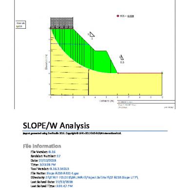
Slope Stability Analysis
March 2021 0
12-01 Slope Monitoring Methods
January 2021 0More Documents from "jayuna1609"
Slope Stability.pdf
February 2021 0
Bechtel Presentation
February 2021 0
Steel-detailing-guide-sample-version.pdf
January 2021 0
Gearbox Design
January 2021 1
A202 Co Kim Cham Vs. Valdez Tan Keh
March 2021 0