Ch3 Bearing Capacity Of Shallow Foundations (72-164).pdf
This document was uploaded by user and they confirmed that they have the permission to share it. If you are author or own the copyright of this book, please report to us by using this DMCA report form. Report DMCA
Overview
Download & View Ch3 Bearing Capacity Of Shallow Foundations (72-164).pdf as PDF for free.
More details
- Words: 27,381
- Pages: 93
Loading documents preview...
CHAPTER
3
BEARING CAPACITY OF SHALLOW FOUNDATIONS 3.1 MODES OF FAILURE Failure is defined as mobilizing the full value of soil shear strength accompanied with excessive settlements. For shallow foundations it depends on soil type, particularly its compressibility, and type of loading. Modes of failure in soil at ultimate load are of three types; these are as shown below in Fig.(3.1). Characteristics
Mode of Failure (i) General Shear Failure B
Load/ unit area, q
qult.
Failure Surface
Settlement
(ii) Local Shear Failure B
Load/ unit area, q
qult.(1) qult.
Failure Surface
Settlement
Typical Soils
Well defined continuous slip surface up to ground level, Heaving occurs on both sides with final collapse and tilting on one side, Failure is sudden and catastrophic, Ultimate value is peak value.
Low compressible soils, Very dense sands, Saturated clays (NC and OC), Undrained shear (fast loading).
Well defined slip surfaces only below the foundation, discontinuous either side, Large vertical displacements required before slip surfaces appear at ground level, Some heaving occurs on both sides with no tilting and no catastrophic failure, No peak value, ultimate value not defined.
Moderate compressible soils, Medium dense sands,
Well defined slip surfaces only below the foundation, non of either side, Large vertical displacements produced by soil compressibility, No heaving, no tilting or catastrophic failure, no ultimate value.
High compressible soils Very loose sands, Partially saturated clays, NC clay in drained shear (very slow loading), Peats.
(iii) Punching Shear Failure B
Load/ unit area, q
qult.(1) qult. Failure Surface
Surface footing
Settlement
qult.
Fig.(3.1): Modes of failure in soil.
Foundation Engineering for Civil Engineers
Chapter 3: Bearing Capacity of Shallow Foundations
3.2 BEARING CAPACITY CLASSIFICATION
Gross Bearing Capacity ( q gross ): It is the total unit pressure at the base of footing
which the soil can take up.
P G.S.
q D f .
Do
Df
t B
q gross = total pressure under the base of footing = Pfooting / area.of .footing . where Pfooting p.(column .load ) + own wt. of footing + own wt. of earth fill over the footing.
q gross (P s .D o .B.L c .t.B.L) / B.L
q gross
P s .D o c .t ……………..……………..……….(3.1) B.L
Ultimate Bearing Capacity ( q ult. ): It is the maximum unit pressure or the maximum
gross pressure that a soil can stand without shear failure.
Allowable Bearing Capacity ( q all. ): It is the ultimate bearing capacity divided by a
reasonable factor of safety.
q all.
q ult. .......................................…........……………….........(3.2) F.S
Net Ultimate Bearing Capacity: It is the ultimate bearing capacity minus the vertical
pressure that is produced on horizontal plain at level of the base of the foundation by an adjacent surcharge. q ult.net q ult. D f . …..…..….……………..…………..…….(3.3)
Net Allowable Bearing Capacity ( q all. net ): It is the net safe bearing capacity or the
net ultimate bearing capacity divided by a reasonable factor of safety.
q ult. D f . ..….......……………….........(3.4) F.S
Approximate:
q all. net
q ult. net
Exact:
q all. net
q ult. D f . ..................…….......……………….........(3.5) F.S
F.S
73
Foundation Engineering for Civil Engineers
Chapter 3: Bearing Capacity of Shallow Foundations
3.3 FACTOR OF SAFETY FOR BEARING CAPACITY The choice of factor of safety (F.S.) depends on many factors such as: 1. The variation of shear strength of soil, 2. Magnitude of damages, 3. Reliability of soil data such as uncertainties in predicting the q ult. by the theoretical or empirical methods, 4. Changes in soil properties due to construction operations, 5. Relative cost of increasing or decreasing F.S., and 6. The importance of the structure, differential settlements and soil strata underneath the structure. The general values of safety factor used in design of footings are 2.5 to 3.0. The upper value (3.0) is normally used for normal design load in service conditions and the lower value (2.5) is used for maximum or transient loading conditions such as wind load or earthquakes.
3.4 BEARING CAPACITY REQUIREMENTS Three requirements must be satisfied in determining bearing capacity of soil. These are: (1) Adequate depth; the foundation must be deep enough with respect to environmental effects; such as: Depth of frost penetration, Depth of seasonal volume changes in the soil, To exclude the possibility of erosion and undermining of the supporting soil by water and wind currents, and To minimize the possibility of damage by construction operations, (2) Tolerable settlements, the bearing capacity must be low enough to ensure that both total and differential settlements of all foundations under the planned structure are within the allowable values, (3) Safety against failure, this failure is of two kinds: The structural failure of the foundation; which may occur if the foundation itself is not properly designed to sustain the imposed stresses, and The bearing capacity failure of the supporting soils.
3.5 FACTORS AFFECTING BEARING CAPACITY 1. 2. 3. 4. 5. 6.
Type of soil (cohesive or cohesionless), Physical features of the foundation; such as size, depth, shape, type, and rigidity, Total and differential settlements that the structure can stand, Physical properties of soil; such as density and shear strength parameters, The water table condition, and Original stresses.
74
Foundation Engineering for Civil Engineers
Chapter 3: Bearing Capacity of Shallow Foundations
3.6 METHODS OF DETERMINING BEARING CAPACITY 3.6.1 BEARING CAPACITY TABLES The bearing capacity values can be found in certain tables presented in building codes, soil mechanics and foundation books; such as that shown in Table (3.1). They are based on experience and can be only used for preliminary design of light and small buildings as a helpful indication; however, they should be followed by the essential laboratory and field soil tests. Table (3.1) neglects the effect of the following items: (i) underlying strata, (ii) size, shape and depth of footings, (iii) type of the structures supported by the footings, (iv) absence of specification of the physical properties of the soil in question, and (v) the assumption that the ground water table level is at foundation level or with depth less than width of footing. Therefore, if water table rises above the foundation level, the hydrostatic water pressure force which affects the base of foundation should be taken into consideration. Table (3.1): Bearing capacity values according to building codes. Soil type
Description
Rocks
1. bed rocks. 2. sedimentary layer rock (hard shale, sand stone, siltstone). 3. shest or erdwas. 4. soft rocks.
Cohesionless soil 1. well compacted sand or sand mixed with gravel. 2. sand, loose and well graded or loose mixed sand and gravel. 3. compacted sand, well graded. 4. well graded loose sand. Cohesive soil
1. 2. 3. 4. 5. 6. 7.
very stiff clay stiff clay medium-stiff clay low stiff clay soft clay very soft clay silt soil
Bearing pressure (kN/m2) 70 30
Unless they are affected by water. 20 13 Dry
submerged
3.5-5.0
1.75-2.5
1.5-3.0
0.5-1.5
1.5-2.0
0.5-1.5
0.5-1.5
0.25-0.5
2-4 1-2 0.5-1 0.25-0.5 up to 0.2 0.1-0.2 1.0-1.5
3.6.2 FIELD LOAD TEST This test is fully explained in (section 2.11 − Chapter 2).
75
Notes
Footing width 1.0 m.
It is subjected to settlement due to consolidation
Foundation Engineering for Civil Engineers
Chapter 3: Bearing Capacity of Shallow Foundations
3.6.3 BEARING CAPACITY EQUATIONS Several bearing capacity theories were proposed for estimating the ultimate bearing capacity of shallow foundations. A summary of some important works developed so far is as follows:(1) PRANDTL, 1921; REISSNER, 1924 ANALYSES Fig.(3.2) shows the Prandtl theory of rupture under line loading. It was based on long metal plate as a continuous or strip footing with the following assumptions: The surface of plate is very smooth, L/B is (i.e., strip footing), The load is applied axially to the center of plate, There is no friction between soil and plate, The failure pattern consists of three zones; zone (I) is an active Rankine zone, which pushed the radial Prandtl zone (II) sideways and the passive Rankine zone (III) in an upward direction. The weights of the three soil zones are neglected. The lower boundary acde of the displaced soil mass is composed of two straight lines ac and de inclined at (45 / 2) and (45 / 2) , respectively to the horizontal. The shape of the connecting curve cd depends on the angle and on the ratio ( .B / q ). Hence, when .B / q = 0 (weightless soil), the curve becomes a logarithmic spiral but if ( 0 ), it degenerates into a circle. B qult.
b
a 45 − Φ/2
𝜶 = 45 + Φ/2
45 − Φ/2
I
III II
e
III II
c
d
Fig.(3.2): Prandtl theory of rupture under line loading.
Under the assumption that 𝛼 = (45 / 2) , the following bearing equations were obtained:(i)
Prandtl and Reissner, 1921−1924 Analyses:
(ii)
Caquot and Kerisel, 1953 Analyses:
(for weightless soil; 0 ): q ult. cN c qN q ………..…….….…………..……………..(3.6) (for cohesionless soil; c = 0 without overburden; q = 0 ): 1 q ult. B..N .……....……….…………..………………..(3.7) 2
76
Foundation Engineering for Civil Engineers
Chapter 3: Bearing Capacity of Shallow Foundations
Now summing Eqs.(3.6 and 3.7) gives (for c 0,..q 0,..and.. 0 ): 1 q ult. cN c qNq .B..N ....……..……….………...…..(3.8) 2 where, N c , N q , and N are bearing capacity factors defined as:
N q e . tan tan2 (45 / 2) ; same as Meyerhof, Hansen, and Vesic
N c ( N q 1). cot ;
same as Meyerhof, Hansen, and Vesic
N 2.(Nq 1). tan ;
same as Vesic
Eq.(3.8) is known as (Buisman, 1940 - Terzaghi, 1943 bearing capacity equation for strip footing). But, it leads to an errors on the safe side, not exceeding 20% for 20 40 , while equal to zero for 0 . (2) TERZAGHI'S BEARING CAPACITY EQUATION Terzaghi's equation was produced from a slightly modification of the bearing capacity theory developed by Prandtl using the following assumptions: (a) The footing is continuous footing L/B and the soil is homogenous, (b) The base of footing is rough; there is a friction between footing and soil, (c) The shear strength of soil located above the base the footing is neglected, and could be replaced by a surcharge (q = D f . ), and (d) The load is applied axially at the center of the footing (centric load). Referring to Fig.(3.3), the failure area in the soil under the foundation can be divided into three major zones. These are: (1) Zone cba: this is a triangular elastic zone located immediately below the bottom of the foundation. The inclination of sides ac and ab of the wedge with the horizontal is ( ); the soil friction angle, while most other theories use ( 45 / 2 ), (2) Zone cad: this zone is the Prandtl radial shear zone, and (3) Zone cde: this zone is the Rankine passive zone. Qult. B c e
b
Cd
Cd
a
Pp
Pp
Forces on the elastic wedge.
Fig.(3.3): Failure surface in soil at ultimate load for a continuous rigid foundation as assumed by Terzaghi, Meyerhof, and Hansen, (after Das, 2009). 77
Foundation Engineering for Civil Engineers
Chapter 3: Bearing Capacity of Shallow Foundations
Terzaghi's bearing capacity equation is developed by summing all vertical forces on the wedge cba shown in Fig.(3.3) and equating the sum to zero. The wedge cba will be in equilibrium at failure under the following forces:(1) The total ultimate load ( Q ult. ) acting vertically downward.
Qult. q ult..( B) ….……………..…………………………...….................…..(3.9) (2) The weight of the wedge cba: 1 B 1 wt. of cba = . B.( tan ) .B2 . tan .………………....……..………(3.10) 2 2 4 This weight acting downward and can be neglected due to its very small value. (3) The resultant passive earth pressure Pp acting on the faces ab and ac and inclined at an
angle to the normal to these faces. (4) The cohesive force C d acting along the faces ab and ac. Taking into account the above forces, the equation of equilibrium can be written as: 1 Q ult. .B 2 tan 2{Pp C d . sin ) .…..….……...……..….……..………(3.11) 4
B/2 ) ; where c is soil cohesion acting along the faces ab and ac, and the cos Pp Pp Ppc Ppg resultant Pp can be divided into three components as: But,
C d c.(
where, Pp is the passive earth pressure produced by the weight of (caed) zone, Ppc is the passive earth pressure produced by cohesion (c), and Ppg is the passive earth pressure produced by surcharge (q). 1 B Q ult. .B2 tan 2{Pp Ppc Ppg c. . tan ) .….….…..….…………(3.12) 4 2 2Ppc 2Ppg 2Pp 1 Q ult. B.( B.. tan ) ( c. tan ) ………….………(3.13) 4 B B B 1 Q ult. B. B..N D f ..N q c.N c ……………..………………..………(3.14) 2 1 q ult. cN c .Sc qNq .B..N.S ….…………..…………...……….…..(3.15) or 2 Eq.(3.15) is known as Terzaghi's bearing capacity equation. for any type of footings under general shear failure. where, N c , N q and N are bearing capacity factors Sc and S are shape factors. q̅ is the overburden pressure at foundation level.
78
defined in Tables (3.2 and 3.3).
Foundation Engineering for Civil Engineers
Chapter 3: Bearing Capacity of Shallow Foundations
(3) MEYERHOF'S BEARING CAPACITY EQUATION Meyerhof (1951) proposed a bearing capacity equation similar to that of Terzaghi but included a shape factor S q for the depth term N q , depth factors d i and inclination factors i i for cases where the footing load is inclined from the vertical. Vertical load:
q ult. c.N c .Sc .d c q.N q .Sq .d q 0.5..B.N .S .d .….……..……(3.16)
Inclined load:
q ult. c.N c .d c .i c q.N q .d q .i q 0.5..B.N .d .i
…....................(3.17)
where, N c , N q and N are bearing capacity factors defined by Table (3.2) as:
N q e . tan tan2 (45 / 2) ;
N c ( N q 1). cot ;
N ( N q 1). tan(1.4)
See Table (3.4) for shape, depth and inclination factors.
Note: Up to Df / B 1 (shallow foundations), q ult. from Meyerhof's Eqs.(3.16 or 3.17) is not greatly different from the Terzaghi's value, however, the difference is more pronounced at larger Df / B ratios. (4) HANSEN'S BEARING CAPACITY EQUATION Hansen (1970) proposed the general bearing capacity case. He presented an equation considered as a further extension of Meyerhof's (1951) equation that includes factors for the footing being tilted from horizontal bi and for possibility of the footing being on a slope g i . Hansen’s equation allows any D/B and thus can be used for shallow or deep footings (piles and drilled caissons). Comparing with field results, Hansen’s equation gives more accurate results than those obtained from Terzaghi's equation. (a) for.. 0
q ult. cN cSc d c i c g c b c qN q Sq d q i q g q b q 0.5.B.N S d i g b ………….…..(3.18) (b) for.. 0 (undrained condition; N c 5.14,.N q 1,.N 0 )
q ult. 5.14Su (1 Sc d c i c bc g c ) q ………….…….……..……………...(3.19) where, N c , N q and N are bearing capacity factors defined in Table (3.2) as:
N q e . tan tan2 (45 / 2) ; Same as Meyerhof N c ( N q 1). cot ;
Same as Meyerhof ;
N 1.5( N q 1). tan See Table (3.5) for shape, depth and inclination factors.
79
Foundation Engineering for Civil Engineers
Chapter 3: Bearing Capacity of Shallow Foundations
(5) VESIC'S BEARING CAPACITY EQUATION It is essentially the Hansen equation but with slightly different N and a variation in some of Hansen's i i , b i ..and..g i factors as noted in Table (3.5) with the subscript (V). Any factor is subscripted with (H) can be used for Vesic solution.
Note: Due to scale effects, N and then the ultimate bearing capacity decreases with the increase in the size of foundation. Therefore, Bowles (1996) suggested that for (B > 2m), in any bearing capacity equation of Table (3.2), the term ( 0.5B.N S d ) must be multiplied by a B r 1 0.25 log 2
reduction factor:
; i.e., 0.5B.N S d r
B (m)
2
2.5
3
3.5
4
5
10
20
100
r
1
0.97
0.95
0.93
0.92
0.90
0.82
0.75
0.57
(6) BALLA'S BEARING CAPACITY EQUATION This equation is originally derived for strip footing with ( D f / B 1.5 ) on cohesionless soil or soil with little cohesion. It considers the depth of footing as well as the shearing stress developed along the failure surfaces and the solution generates some very complicated mathematical expressions. However, programming these expressions, a final form of equation can be written as: q ult. cN c qN q b..N
……….…..……….………...…..(3.20)
where, N c , N q and N are bearing capacity factors determined as follows: (1) (2) (3)
Obtain Df / b and c/b , where, b = B/2. With Df / b , c/b , and use Fig.(3.4) to find the factor . With known values of and , enter Fig.(3.5) to determine the bearing capacity factors N c , N q and N , respectively.
80
Foundation Engineering for Civil Engineers
Chapter 3: Bearing Capacity of Shallow Foundations
Table (3.2): Summary of bearing capacity equations by several investigators
(after Bowles, 1996).
Terzaghi (see Table 3.3 for typical values for K P values)
q ult. cNc .Sc qNq 0.5.B..N.S
2[0.75. ( )]. tan 2 180 e Nq ; 2 cos 2 ( 45 / 2)
N
N c ( N q 1). cot ;
tan k P ( 1) 2 cos 2
( 33) where a close approximation of k P 3. tan2 45 . 2 Sc = S =
Strip 1.0
circular 1.3
square 1.3
rectangular (1+ 0.3 B / L)
1.0
0.6
0.8
(1- 0.2 B / L)
Meyerhof (see Table 3.4 for shape, depth, and inclination factors) Vertical load:
qult. c.Nc .Sc .dc q.Nq .Sq .dq 0.5.B..N .S .d
Inclined load:
q ult. c.Nc .dc .ic q.Nq .dq .iq 0.5.B..N .d .i
N q e . tan tan2 (45 / 2) ;
N ( N q 1). tan(1.4)
Hansen (see Table 3.5 for shape, depth, and inclination factors)
For.. 0 :
qult. cNcScdcicgcbc qNqSqdqiqgq bq 0.5.B..N S d i g b
For.. 0 :
q ult. 5.14Su (1 Sc dc ic bc gc ) q
Nq e. tan tan2 (45 / 2) ;
N c ( N q 1). cot ;
N c ( N q 1). cot ;
N 1.5( N q 1). tan
Vesic (see Table 3.5 for shape, depth, and inclination factors) Use Hansen's equations above
N q e . tan tan2 (45 / 2) ;
N c ( N q 1). cot ;
N 2( N q 1). tan
All above bearing capacity equations are based on general shear failure in soil. For Hansen’s and Vesic’s bearing capacity equations, Nc and Nq factors are the same as those of Meyerhof whereas, N is different in all.
81
Foundation Engineering for Civil Engineers
Chapter 3: Bearing Capacity of Shallow Foundations
Table (3.3): Bearing capacity factors of Terzaghi's equation.
,.. deg
Nc
Nq
N
K P
0 5 10 15 20 25 30 34 35 40 45 48 50
5.7 7.3 9.6 12.9 17.7 25.1 37.2 52.6 57.8 95.7 172.3 258.3 347.5
1.0 1.6 2.7 4.4 7.4 12.7 22.5 36.5 41.4 81.3 173.3 287.9 415.1
0.0 0.5 1.2 2.5 5.0 9.7 19.7 36.0 42.4 100.4 297.5 780.1 1153.2
10.8 12.2 14.7 18.6 25.0 35.0 52.0 82.0 141.0 298.0 800.0
= 1.5 + 1
Table (3.4): Shape, depth and inclination factors of Meyerhof's equation. For
Shape Factors B L
Any
Sc 1 0.2.K P
10
Sq S 1 0.1.K P
0 where,
Depth Factors d c 1 0.2 K P B L
Df B
d q d 1 0.1 K P
Sq S 1.0
Inclination Factors
Df B
dq d 1.0
i c i q 1 90
i 1 i 0
K P tan2 (45 / 2) angle of resultant measured with vertical without a sign. B, L , Df = width, length, and depth of footing.
B Note:- When triaxial is used for plan strain, adjust as: Ps (1.1 0.1 )triaxial L
82
2
R
2
Foundation Engineering for Civil Engineers
Chapter 3: Bearing Capacity of Shallow Foundations
83
Foundation Engineering for Civil Engineers
Chapter 3: Bearing Capacity of Shallow Foundations
Fig.(3.4) Values of ratio for various c / b and Df / b values for Balla’s bearing capacity equation (after Bowles, 1996).
Fig.(3.5) Bearing capacity factors Nc ,..Nq ,..and..N to be used in Balla's equation (after Bowles, 1996).
84
Foundation Engineering for Civil Engineers
Chapter 3: Bearing Capacity of Shallow Foundations
3.7 WHICH EQUATION TO BE USED? The summary of using of all bearing capacity equations is shown in Table (3.6). Of the bearing capacity equations previously discussed, the most widely used equations are Meyerhof's and Hansen's among others. However, Vesic's equation is a suggested method in API manual (American Petroleum Institute, RP2A Manual, 1984). Table (3.6): Uses of bearing capacity equations. Equation
Best for
Terzaghi
Pure cohesive soils where D/B
1 or for a quick estimate of
q ult.
compared with other methods,
Somewhat simpler than Meyerhof's, Hansen's or Vesic's equations; that need to compute shape, depth, inclination, base and ground factors,
Suitable for a concentrically loaded horizontal footing,
Not applicable for columns with moments or tilting forces,
More conservative than other methods.
Any situation depending on user preference with a particular method.
Hansen, Vesic
When base is tilted; when footing is on a slope or when D/B >1.
Balla
Cohesionless soils or soil with little cohesion when D/B
Meyerhof, Hansen, Vesic
1.5.
3.8 SOIL STRENGTH CASES There are three cases usually considered in soil mechanics, which affect the type of shear strength parameters c and to be used in bearing capacity equations; these cases are shown in Table (3.7). Table (3.7): Shear strength parameters according to soil strength cases. Soil Strength Case
Cohesion
Friction
Case (1): Undrained condition in clay (short-term case).
c cu
u 0
Case (2): Drained condition in clay (long-term case).
c c
( 0)
Case (3): Drained condition in sand (short and long term case).
c0
( 0)
The shape, depth, inclination and other factors used in different bearing capacity equations are also dependent on the choice of c and values, so that different factors will be obtained depending on the soil strength case assumed.
85
Foundation Engineering for Civil Engineers
Chapter 3: Bearing Capacity of Shallow Foundations
3.9 CONTACT PRESSURE The pressure acting between a footing's base and the soil below is referred to as contact pressure. Knowledge of contact pressure and associated shear and moment distributions is important in footing design. Contact pressure can be computed using the flexural formula:q
P M x .y M y .x ………………….…..……….………...…..(3.21) A Ix Iy
where, q= P = A= M x ,..M y I x ,..I y
contact preesure, total axial vertical load = D.L. + L.L., area of footing, total moment about respective x and y axes, moment of inertia about respective x and y axes,
x, y = distance from centriod to the point at which the contact pressure is computed along respective x and y axes.
P D.L L.L
P D.L L.L
P D.L L.L
center line center line e
L
P q act . Af
L
e
Or
q min.
L
q min.
center line
q max . (a) Concentric load
q max .
(b) Eccentric load
Fig.(3.6): Contact pressure distribution under footings.
As shown in Fig.(3.6a), if the moments about both x and y axes are zero, then, the contact pressure is simply equal to the total vertical load divided by the footing's area. While in case of moment or (moments), the contact pressure below the footing will be non-uniform (see Fig.3.6b).
86
Foundation Engineering for Civil Engineers
Chapter 3: Bearing Capacity of Shallow Foundations
Assuming that moment is only in (L - direction), due to this moment, there will be a nonuniform contact pressure below the footing under the following three cases: (1)
when e x L / 6 , the resultant of loading passes within the middle third of the footing. Here, there is compression under the footing with maximum pressure on one side and minimum pressure on the other side.
(2)
when e x L / 6 , the resultant of loading passes on edge of the middle third of the footing.
(3)
when e x L / 6 , the resultant of loading is outside the middle third of the footing. Here, there will be a tension under the footing.
Case (1):
When moment in (L- direction only) and e x L / 6
e x = eccentricity =
B.L3 L M ; c ; I ; 12 2 P
M.c 6M ; M = P..e x I B.L2 q max . q min.
B.L P
B.L
6 P.e x
M L/3
P Af
2
B.L
. q max min .
or
P
q act .
P = D.L.+L.L.
L/6 L/6
L/3
L
M.c I
6 P.e x
+
B.L2
M.c I
q min.
P
6.e x 1 B.L L
q max .
When moments (in both directions) and e x L / 6 ; e y B / 6
ex
My P
;
. or q max min .
or
. q max min .
ey P
B.L
y
Mx P
6 P.e x B.L2
My
6 P.e y B 2 .L
ey
B x
P
6.e x 6.e y 1 B.L L B
L
y
87
Mx
ex
x
Foundation Engineering for Civil Engineers
Chapter 3: Bearing Capacity of Shallow Foundations
Case (2): When moment in (L– direction) only and e x L / 6
P= D.L.+L.L.
q max . q min.
ex
P
6.e x P L 2 P 1 = = 1 B.L L B.L L B.L P
6.e x P L 1 = =0 1 B.L L B.L L
L/3
L/6 L/6
L/3
q min. = 0
q max .
Case (3): When moment in (L– direction) only and e x L / 6 P = q . B. L
P = D.L.+L.L. ex
1 q max . .L1 .B ………………………..…...(a) 2 L L e 1 …………………..…………….…...(b) 3 2 2 P From equation (a): q max . ………………(c) L1 .B L From equation (b): L1 3 e x …………....(d) 2 P
Substituting equation (d) into equation (c) gives:
q max .
L/6 L/2
ex
L1/3
q min. = 0
q max .
2. P L 3.B e x 2
L1
P = D.L.+L.L.
3.10 EFFECT OF SOIL COMPRESSIBILITY 1. For clays sheared in drained conditions, Terzaghi (1943) suggested that the shear
strength parameters c and should be reduced as:
c* 0.67c and * tan1(0.67 tan ) ……………...………...…..(3.22) 2. For loose and medium dense sands (when D r 0.67 ), Vesic (1975) proposed:
* tan1(0.67 Dr 0.75D2r ) tan ……………...………...………...(3.23) where, D r is the relative density of the sand, recorded as a fraction. Note: For dense sands ( Dr 0.67 ), the strength parameters need not to be reduced, since the
general shear mode of failure is likely to apply.
88
Foundation Engineering for Civil Engineers
Chapter 3: Bearing Capacity of Shallow Foundations
3.11 EFFECT OF WATER TABLE Generally, the submergence of soils will cause loss of all apparent cohesion, coming from capillary stresses or from weak cementation bonds. At the same time, the effective unit weight of submerged soils will be reduced to about one-half the weight of the same soils above the water table. Thus, through submergence, all the three terms of the bearing capacity (B.C.) equations may be considerably reduced. Therefore, it is essential that the B.C. analysis be made assuming the highest possible groundwater level at the particular location for the expected life time of the structure. W.T.
G.S.
Case (5) D1
W.T. Case (4)
Df D2
B
m
W.T.
W.T. Case (3)
dw
Case (2)
B
W.T.
Case (1)
Case (1): If the water table (W.T.) lies at B or more below the foundation base; no W.T. effect. Case (2): a- (after Meyerhof, 1951): If the water table (W.T.) lies within the depth ( d w
H 0.5B tan(45 / 2) , = submerged unit weight =( sat. w ), d w = depth to W.T. below the base of footing, and m wet = moist or wet unit weight of soil in depth ( d w ).
89
Foundation Engineering for Civil Engineers
Chapter 3: Bearing Capacity of Shallow Foundations
Case (3): If d w = 0 ; the water table (W.T.) lies at the base of the foundation; use Case (4): If the water table (W.T.) lies above the base of the foundation; use: 1 q t .D1(above..W.T.) .D 2 (below..W.T.) and in .B.N term. 2 Case (5): If the water table (W.T.) lies at ground surface (G.S.); use: q .D f and 1 in .B.N term. 2 Notes: 1 .B.N can be ignored for 1. Since in many cases of practical purposes, the term 2 1 conservative results, it is recommended for this case to use in the term .B.N 2 instead of av. since ( av. ( from..Meyerhof ) av. ( from..Bowles ) ) 2. All the preceding considerations are based on the assumption that the seepage forces acting on soil skeleton are negligible. The seepage force adds a component to the body forces caused by gravity. This component acting in the direction of stream lines is equal to (i. w ) , where i is the hydraulic gradient causing seepage.
Problem (3.1): (Contact pressure) Proportion a footing subjected to concentric column load (1600 kN) and to an overturning moment (800 kN-m), if q all. =200 kPa. Solution:
or
My
800 0.5 m ; put q max . q all. of soil 1600 p 1600 3 P 6.e x q max . 1 1 ; 200 = B.L L B.L L
ex
Area Proportion: Choose B and L such that (L/B < 2.0)
L (m) Let, L = 6e = 3 4 5 6 7
B (m)
Area (m2)
5.40 3.50 2.56 2.00 1.63
16.20 14.00 12.80 12.00 11.42
L/B 0.55 < 2.0 1.14 < 2.0 1.95 < 2.0 3.00 > 2.0 4.29 > 2.0
Take L = 5.0 and B = 2.6
Check : L / 6 = 5 / 6 = 0.83m > e x = 0.5m The load is within the middle 3rd.
90
(O.K.)
Foundation Engineering for Civil Engineers
Chapter 3: Bearing Capacity of Shallow Foundations
Problem (3.2): (Effect of water table) A (1.2m x 4.2m) rectangular footing is placed at a depth of ( D f =1m) below the G.S. in
clay soil with u 0 , 18 kN/m3, C u 22 kN/m2. Find the allowable maximum load which can be applied under the following conditions: (a) W.T. at base of footing with sat 20 kN/m3, (b) (c)
W.T. at 0.5m below the surface and sat 20 kN/m3, If the applied load is 400kN and the W.T. at the surface what will be the factor of safety of the footing against B.C. failure?
Pall. ? G.S.
= 18 kN/m3 D f =1.0m Solution: (a)
c 22 kN/m2 B =1.2m
u 0
W.T. at base of footing:
L/B = 4.2/1.2 = 3.5 < 5 rectangular footing, D/B = 1/1.2 = 0.833 < 1.0 shallow footing; therefore Terzaghi's equation is applicable. Terzaghi's equation is:
1 q ult. cN c .Sc qNq .B..N.S 2 Bearing capacity factors: From Table (3.3) for 0 : N c 5.7 , Nq 1.0 , and N 0 B
B
Shape factors: From Table (3.2) for rectangular footing: Sc (1 0.3 ) ; S (1 0.2 ) L L
q ult. (22)(5.7)(1 + 0.30
1 .2 ) + (1.0)(18)(1) 4 .2
+ 0.5(1.2)(20-10)(0)(1 - 0.20
1 .2 )= 154.148 kN/m2 4 .2
q all. = 154.148 /3 = 51.388 kN/m2 Pall. = 51.388(1.2)(4.2) = 258.970 kN (b)
W.T. at 0.5m below the ground surface:
q t .D1(above..W.T.) .D 2 (below..W.T.) D1 0.5 and D 2 0.5 ; q 18.(0.5) (20 10)(0.5) 14 kN/m2
q ult. (22)(5.7)(1 + 0.30
1 .2 1 .2 ) + (14)(1) + 0.5(1.2)(20-10)(0)(1-0.20 )= 150.148 kN/m2 4 .2 4 .2
q all. = 150.148 /3 = 50.049 kN/m2 Pall. = 50.049(1.2)(4.2) = 252.249 kN
91
Foundation Engineering for Civil Engineers (c)
Chapter 3: Bearing Capacity of Shallow Foundations
If the applied load is 400 kN and the W.T. at the surface what will be the factor of safety of the footing against B.C. failure?.
Pall. = 400 kN; q all. = 400/(1.2)(4.2)= 79.36 kN/m2; q D f . =(1)(20-10)=10 kN/m2 1 .2 1 .2 ) + (10)(1) + 0.5(1.2)(20-10)(0)(1 - 0.20 )= 146.14 kN/m2 q ult. (22)(5.7)(1 + 0.30 4 .2 4 .2 q 146.14 SF ult. 1.8 q all. 79.36
Problem (3.3): (Effect of water table) A vertically and concentrically loaded (2.5m x 2.5m) square footing is to be placed on a cohesionless soil as shown below. What is the allowable B.C. using the Hansen’s equation and a safety factor (SF) = 2.0? P G.S.
D f =1.1m 2.5m x 2.5m
1.95m
m = 18.1 kN/m3 c 0 kN/m2 tr. 35 w 10% Gs 2.68
W.T.
sat = ?
Solution:
m 18.1 = 16.45 kN/m3 1 1 0.10 d 16.45 0.626 m3 = Vs G s . w (2.68)(9.81) Vv 1.0 Vs 1 0.626 0.374 m3 The saturated unit weight is the dry weight + weight of water in voids. sat. d Vv . w = 16.45 + 0.374(9.81) = 20.12 kN/m3 d
From the figure d w 0.85m and H 0.5B tan(45 / 2) = 2.4m ( d w H ); i.e., the water table (W.T.) lies within the wedge zone H 0.5B tan(45 / 2) . 1 Therefore, use av. in the term .B.N : 2 d av. (2H d w ) w . wet (H d w ) 2 2 2 H H 0.85 (20.12 9.81) av. (2)(2.4) 0.85) (18.1) (2.4 0.85)2 14.85 kN/m3 2 2 2.4 2.4
92
Foundation Engineering for Civil Engineers
Chapter 3: Bearing Capacity of Shallow Foundations
Using Hansen's equation:
q ult. cN cSc d c i c g c b c qN q Sq d q i q g q b q 0.5.B.N S d i g b
Since, c = 0, any factors with subscript c do not need computing. Also, all g i ..and..b i factors are 1.0; with these factors identified the Hansen's equation simplifies to: q ult. qN q Sq d q 0.5 av. .B.N S d No need to compute ps , since footing is square. Bearing capacity factors from Table (3.2): For 35 :
Nq e. tan .. tan2 (45 / 2) 33.3
and N 1.5( Nq 1) tan 33.9
B B tan 1.7 and S 1 0.4 0.6 L L D Depth factors from Table (3.5): d q 1 2 tan (1 sin ) 2 , and d 1.0 B d q 1 2 tan 35(1 sin 35) 2 (1.1 / 2.5) 1.11 , q ult. (1.1)(18.1)(33.3)(1.7)(1.11)+ 0.5(14.85)(2.5)(33.9)(0.6)(1.0)= 1617 kN/m2 q all. =1617/2 = 808.5 kN/m2 Shape factors from Table (3.5): Sq 1
Note:
808.5 kN/m2 is very large bearing pressure; since in most cases, the allowable bearing capacity does not exceed 500 kN/m2.
Problem (3.4): (Allowable net bearing capacity) Determine the allowable net bearing capacity of a strip footing using Terzaghi’s and Hansen’s equations if c = 0, 30 , D f = 1.0m , B = 1.0m , soil 19 kN/m3, the water table is at ground surface, and SF=3. Solution: (a)
Using Terzaghi's equation:
1 q ult. cN c .Sc qN q .B..N.S 2 Shape factors From Table (3.2): For strip footing: Sc S 1.0 Bearing capacity factors From Table (3.3): For 30 : Nq 22.5, and q ult. 0 + 1.0 (19-9.81)(22.5)(1.0) + (0.5)(1)(19-9.81)(19.7)(1.0) = 297 kN/m q all. =297/3 = 99 kN/m2 qall.(net ) qall. Df . 99 – (1)(19 – 9.81) 90 kN/m2
93
N 19.7 2
Foundation Engineering for Civil Engineers (b)
Chapter 3: Bearing Capacity of Shallow Foundations
Using Hansen's equation:
For.. 0 :
q ult. cN cSc d c i c g c b c qN q Sq d q i q g q b q 0.5.B.N S d i g b
Since c = 0, factors with subscript c do not need computing. Also, all g i ..and..b i factors are 1.0; with these factors identified the Hansen's equation simplifies to: q ult. qN q Sq d q 0.5 .B.N S d
for........... 34 ..use.. ps tr From Table (3.5): ...use...ps 1.5tr 17 for L/B 2 ..use.. ps 1.5tr 17 .....ps (1.5)(30) – 17 = 28 Bearing capacity factors from Table (3.2): For 28 :
Nq e. tan .. tan2 (45 / 2) 14.7 ,
Shape factors from Table (3.5):
N 1.5( Nq 1) tan 10.9
Sq S 1.0,
Df B 1 dq 1 2. tan 28(1 sin 28)2 1.29 1
Depth factors from Table (3.5): dq 1 2 tan (1 sin )2
and
d 1.0
q ult. 1.0 (19-9.81)(14.7)(1.29) + 0.5(1)(19 – 9.81)(10.9)(1.0) = 224.355 kN/m2 q all. = 224.355/3 = 74.785 kN/m2
qall.(net ) 74.785 – (1)(19 – 9.81) 66 kN/m2
Problem (3.5): (Ultimate bearing capacity) A footing load test produced the following data: D f = 0.5m, B = 0.5m, L = 2.0m, soil 9.31 kN/m3, c = 0 kN/m2, tr 42.5 , Qult.(measured ) = 1863 kN, and q ult.(measured ) = 1863/(0.5)(2.0) = 1863 kN/m2. Compute q ult. using Hansen's and Meyerhof's equations and compare the computed values with those measured. Solution: (a)
Using Hansen's equation:
Since c = 0, and all g i ..and..b i factors are 1.0; Hansen's equation simplifies to: q ult. qN q Sq d q 0.5 .B.N S d From Table (3.5): L / B = 2 / 0.5 = 4 > 2 1.5 (42.5) – 17 = 46.75 ;
Take
....use..... ps 1.5tr 17 ,
47
94
Foundation Engineering for Civil Engineers
Chapter 3: Bearing Capacity of Shallow Foundations
Bearing capacity factors from Table (3.2): For 47 :
Nq e. tan .. tan2 (45 / 2) 187.2 ,
N 1.5( Nq 1) tan 299.5
Shape factors from Table (3.5): B 0.5 Sq 1 tan 1 tan 47 1.27, L 2.0 B 0.5 S 1 0.4 1 0.4 0.9 L 2.0 Depth factors from Table (3.5): dq 1 2 tan (1 sin )2
Df B
0.5 1.155 , d 1.0 0.5 q ult. 0.5 (9.31)(187.2)(1.27)(1.155) + 0.5(9.31)(0.5)(299.5)(0.9)(1.0) = 1905.6 kN/m2 versus 1863 kN/m2 measured. d q 1 2 tan 47(1 sin 47) 2
(b)
Using Meyerhof's equation: From Table (3.2) for vertical load with c = 0:
q ult. qN q Sq d q 0.5 .B.N S d
B 0 .5 From Table (3.4): ps (1.1 0.1 ) tr = (1.1 - 0.1 )42.5 = 45.7; L 2 .0 Bearing capacity factors from Table (3.2): For 46 :
Nq e. tan .. tan2 (45 / 2) 158.5 ,
Take 46
N ( Nq 1) tan(1.4.) 328.7
Shape factors from Table (3.4): K p tan 2 (45 / 2) =6.13
Sq S 1 0.1.K p
B 0.5 1 0.1(6.13) 1.15 L 2.0
Depth factors from Table (3.4):
Df 0.5 1 0.1(2.47) 1.25 B 0.5 q ult. 0.5(9.31)(158.5)(1.15)(1.25) + 0.5(9.31)(0.5)(328.7)(1.15)(1.25) = 2160.4 kN/m2 K p 2.47 ,
dq d 1 0.1. K p
versus 1863 kN/m2 measured. Both Hansen's and Meyerhof's equations give overestimated q ult. compared with that measured.
Problem (3.6): (Ultimate bearing capacity) A series of large-scale footing B.C. tests were performed on soft Bangkok clay. One of the tests consisted of (1.05m) square footing at ( D f =1.5m). At (25 mm) settlement the load obtained was approximately (14.1 ton) from the load-settlement curve. Unconfined compression and vane shear tests gave unconfined strength values as follows: LL 80%, , PL 35% , q u 3 Tons/m2, and Su,Vane 2.4 Tons/m2. Compute q ult. using Hansen’s equation and compare it with the load test value of (14.1 ton).
95
Foundation Engineering for Civil Engineers
Chapter 3: Bearing Capacity of Shallow Foundations
Solution:
Obtain N,.Si ,..and..d i factors, since 0 for soft clay (in unconfined compression test), N c 5.14 and N q 1.0 . Using Fig.(2.27a) for PI = 45% obtain a reduction factor . 0.8. S u , desgin ...S u , Vane = 0.8(2.4) = 1.92 ton/m2.
D B 1 1.5 0.2 0.2 , and d c 0.4 tan 1 0.4 tan 1 0.38 (D >B) B L 1 1.05 From Table (3.2): for.. 0 (undrained condition; N c 5.14,.N q 1,.N 0 ) Sc 0.2
q ult. 5.14Su (1 Sc d c ic bc g c ) q Neglecting ( i c , bc ,..and..g c ) and q.N q since there was probably operating space in the footing excavation, Hansen's equation will be: qult. 5.14.Su (1 Sc dc ) From Vane shear test: q ult. = 5.14(1.92)(1+ 0.2 + 0.38) = 15.6 ton/m2 From load test:
q actual
14.1 12.8 ton/m2 (1.05)(1.05)
If we use; S u q u / 2 , we obtain: From unconfined compressive test: q ult.
1.5 (15.6) 12.2 ton/m2 1.92
Problem (3.7): (Allowable bearing capacity for cohesive soil) A series of q u tests in the zone of interest (from SPT samples) of a boring log give an average value of 200 kPa. Estimate q all for square footings located at somewhat uncertain depths of unknown B dimensions using both Meyerhof's and Terzaghi's equations if SF = 3.0. Solution:
This Problem illustrates the most common method for obtaining q all of cohesive soils in case of limited data. (a) Using Meyerhof's equation: q ult. cN cSc d c qN q Sq d q 0.5 .B.N S d From Table (3.2):
For.. 0 :
Nc 5.14,...Nq 1,...and...N 0
From Table (3.4): K p tan 2 (45 / 2) =1 ; Sc 1 0.2K p Sq S 1.0 ; d q d 1.0 ;
q ult. cN c Sc qN q
B =1.2 (for square footing), L
q q 1 q qall. ult. 1.2 u (5.14) 1.03q u 0.3q 3 2 3 3
96
Foundation Engineering for Civil Engineers (b)
Chapter 3: Bearing Capacity of Shallow Foundations
Using Terzaghi's equation: From Table (3.2): q ult. cN c Sc qN q 0.5 .B.N S
From Table (3.3): For.. 0 : Nc 5.7 , N q 1 and N 0 ; Sc 1.3 (square footing) q q 1 q q all. ult. 1.3 u (5.7) 1.24q u 0.3q 3 2 3 3 It is common to neglect 0.3q and note that 1.03 or 1.24 is sufficiently close to 1.0 (and is conservative) to take the allowable bearing pressure as:
qall. qu 200.kPa
or
q ult. cN c 3q u
Note: The use of q all. q u for the allowable bearing pressure is nearly universal when
SPT samples are used for q u , since these samples are in very disturbed state. However, this method of obtaining q all. is not recommended when ( q u 75.kPa ), and in these cases S u should be determined from samples of better quality than those of SPT samples.
Problem (3.8): (Allowable bearing capacity of tilted base footing ) A (2.0m x 2.0m) square footing has the geometry and load as shown in figure below. Is the footing adequate with a SF = 3.0?. P G.S. Df = 0.3m
H P = 600 kN H = 200 kN
B
10
B = 2m
= 17.5 kN/m3 c = 25 kN/m2, 25
Solution:
We can use either Hansen's, or Meyerhof's or Vesic's equations. An arbitrary choice is Hansen's method.
Check Sliding Stability:
Use
2 2 ; Ca c 3 3
and Af (2)(2) 4m2
2 2 H max . Af Ca V tan (2)(2)( 25) 600 tan 25 246.3 kN 3 3 H 246.3 Fs(slididing) max . 1.2 1.5 (Not safe for sliding), therefore, increase (B) H 200 301.1 Try B x B = 2.7m x 2.7m , Fs(slididing) 1.5 1.5 (O.K.) 200
97
Foundation Engineering for Civil Engineers
Chapter 3: Bearing Capacity of Shallow Foundations
Bearing Capacity By Hansen's Equation:
With inclination factors all..Si 1.0 q ult. cN c .dc .ic .bc qNq .dq .iq .bq 0.5.B.N .d .i .b .r Bearing capacity factors from Table (3.2):
N c ( N q 1). cot , N q e . tan .. tan 2 (45 / 2) , N 1.5( N q 1) tan For 25 : N c 20.7 , N q 10.7 , N 6.8 Depth factors from Table (3.5):
For Df = 0.3m, and B = 2.7m: Df / B = 0.3/2.7 = 0.11 < 1.0 (shallow footing) D d c 1 0.4 f 1 0.4(0.11) 1.044 B D d q 1 2 tan (1 sin )2 f 1 0.311(0.11) 1.034 , d 1.0 B Inclination factors from Table (3.5):
0.5H 0.5(200) )5 (1 )5 0.587 V Af .c. cot 600 (2.7)(2.7)(25) cot 25 (1 iq ) 1 0.587 ic iq 0.587 0.544 ( N q 1) 10.7 1 iq (1
5
5
(0.7 / 450) H (0.7 10 / 450)200 1 for.. 0 : i 1 0.479 V Af .c. cot 600 (2.7)(2.7)( 25) cot 25 B 2.7 r 1 0.25 log 1 0.25 log 0.967 2 2 Base factors from Table (3.5):
bc 1
10 (10)( / 180) 0.175.(in..radians )
10 1 0.93 147 147
bq e2 tan e2(0.175) tan 25 0.85
b e2.7 tan e2.7(0.175) tan 25 0.80
q ult. 25(20.7)(1.044)(0.544)(0.93) + 0.3(17.5)(10.7)(1.034)(0.587)(0.85) + 0.5(17.5)(2.7)(6.8)(1)(0.479)(0.80)(0.967) = 361.843 kN/m2 q ult.( net ) 361.843 0.3(17.5) S.F. 4.3 > 3.0 (O.K.) 600 q all (2.7)( 2.7)
98
Foundation Engineering for Civil Engineers
Chapter 3: Bearing Capacity of Shallow Foundations
3.12 FOOTINGS WITH INCLINED OR ECCENTRIC LOADS 3.12.1 FOOTINGS WITH INCLINED LOAD If a footing is subjected to an inclined load Q (see Fig.(3.7)), the inclined load is resolved into vertical and horizontal components. The vertical component Q v is then used for bearing capacity analysis in the same manner as described previously (Table 3.2). After the bearing capacity has been computed by the normal procedure, it must be corrected by the R i factor using Fig.(3.7) as:
or
q ult.(inclined..load) q ult.( vertical ..load) ..R i
………………………...(3.25)
In this case, Meyerhof's bearing capacity equation for inclined load shown in Table (3.2) can be used directly: q ult. (inclined..load) cN c d c i c qN q d q i q 0.5 .B.N d i ……….(3.26)
(a) Horizontal foundation
(b) Inclined foundation
Fig.(3.7): Inclined load reduction factors.
Also, in this case, the footings stability with regard to the inclined load's horizontal component must be checked by calculating the factor of safety against sliding as: H Fs (slididing) max . …………………………….…...………….…...(3.27) H where, H = the inclined load's horizontal component, Hmax . Af .Ca tan …. for ( c ) soils; or
99
Foundation Engineering for Civil Engineers
Chapter 3: Bearing Capacity of Shallow Foundations
H max . A f .C a ……….….. for the undrained case in clay ( u 0 ); or H max . tan ……….…. for sand and the drained case in clay ( c 0 ). Af effective..area B.L C a adhesion .C u where... 1.0 ….for soft to medium clays; and . 0.5 …..for stiff clays, = the net vertical effective load = Q v D f . ; or (Q v D f .) u.Af (if the water table lies above foundation level) = the skin friction angle, which can be taken as equal to ( ),and u = the pore water pressure at foundation level.
3.12.2 FOOTINGS WITH ECCENTRIC LOAD Eccentric load results from loads applied somewhere other than the footing's centroid or from applied moments, such as those resulting at the base of a tall column from wind loads or earthquakes on the structure. Fig.(3.8) shows the slip patterns under eccentric loads. It is clear that the side AC of the wedge ABC assumes a shape of a circle, with its center which coincides with the center of rotation of the footing. But, when ( e B / 4 ), the center of rotation remains on the side of the footing opposite to the load (see Fig.(3.8a)). While at ( e B / 4 ) the center of rotation is exactly under the footing edge, moving for larger (e) towards the axis of the footing and causing uplift of its less loaded side (see Fig.(3.8b)). However, to provide adequate SF(against ...lifting ) of the footing edge, it is recommended that the eccentricity ( e B / 6 ).
Fig.(3.8): Theoretical slip patterns under eccentric loads
(after Das, 2009).
100
Foundation Engineering for Civil Engineers
Chapter 3: Bearing Capacity of Shallow Foundations
Footings with eccentric loads can be analyzed for bearing capacity by two methods: (1)
Concept of useful width: In this method, only that part of the footing that is symmetrical with regard to the load is used to determine bearing capacity by the usual method, with the remainder of the footing being ignored. Thus, in Fig.(3.9) with the (eccentric) load applied at the point indicated, for a rectangular footing, the effective or shaded area is symmetrical with regard to the load, and it is used to determine bearing capacity. Whereas, the effective area for circular footing is computed by locating ( e x ) on any axis (x-axis shown) and producing a centrally located area abcd constructed as shown in Fig.(3.9). Then, area of abc is computed as a segment of a circle which is doubled to give the centrally area abcd ( Af B.L Area of abcd).
First, computes eccentricity and adjusted dimensions: My
Mx ; B B 2e y ; Af A B.L V V Second, calculates q ult. from Meyerhof's, or Hansen's, or Vesic's equations (Table 3.2) 1 using B in the ( B..N ) term and B or/ and L in computing the shape factors and 2 the actual B in computing depth factors.
ex
;
L L 2e x ;
ey
Fig.(3.9): Effective footing dimensions when footing is eccentrically loaded for both rectangular and round bases.
(2) Application of reduction factors: First, compute the bearing capacity by the normal procedure (using equations of Table 3.2), assuming that the load is applied to the centroid of the footing. The computed value is then corrected for eccentricity by a reduction factor ( R e ) obtained from Fig.(3.10) or from Meyerhof's reduction equations as:
101
Foundation Engineering for Civil Engineers
Chapter 3: Bearing Capacity of Shallow Foundations
R e 1 - 2(e/B) …........for.. cohesive.. soil
………….………….……….(3.28) R e 1 - e/B …..... ....for..cohesionles s..soil q ult.(eccentric ) q ult.(concentric ) × 𝑹𝒆 .………….……....…......…..…..(3.29)
Fig.(3.10): Eccentric load reduction factors.
Problem (3.9): (Footing with inclined load) A square footing of (1.5m x1.5m) is subjected to an inclined load as shown in the figure below. What is the factor of safety against bearing capacity (use Terzaghi's equation).
30
G.S.
D f = 1.5m
180 kN
= 20 kN/m3 B = 1.5m 4m
q u 160 kPa
W.T.
Solution: Bearing capacity By Terzaghi's equation:
1 q ult. cN c .Sc qN q .B..N.S 2 Shape factors from Table (3.2): For square footing Sc 1.3;...S 0.8 , c q u / 2 = 80 kPa
102
Foundation Engineering for Civil Engineers
Chapter 3: Bearing Capacity of Shallow Foundations
Bearing capacity factors from Table (3.3):
For u 0 :
Nc 5.7 , N q 1.0 , N 0
q ult.( vertical .load) 80(5.7)(1.3)+20(1.5)(1.0) + 0.5(1.5)(20)(0)(0.8) = 622.8 kN/m2 From Fig.(3.7) with 30 and cohesive soil: the reduction factor for the inclined load is 0.42. q ult.(inclined.load) = 622.8(0.42) = 261.576 kN/m2
Q v Q. cos 30 = 180 (0.866) = 155.88 kN q 261.576 Factor of safety (against bearing capacity failure) ult . 3.77 155.88 q act. (1.5)(1.5)
Check for sliding:
H max . Af .C a tan =(1.5)(1.5)(80) + (180)(cos30)(tan0)=180 kN H = Q h Q. sin 30 = 180 (0.5) = 90 kN H 180 2.0 Factor of safety (against sliding) max. (O.K.) H 90
Problem (3.10): (Footing with eccentric load in one direction) A (1.5m x1.5m) square footing is subjected to eccentric load as shown in the figure below. What is the safety factor against bearing capacity failure (use Terzaghi's equation) using: (a) The concept of useful width, and (b) Meyerhof's reduction factors. P = 330 kN G.S. 1.2m
= 20 kN/m3 q u = 190 kN/m2
Centerline of footing e x =0.18m
1.5m
B 1.5-2(0.18)=1.14m 1.5m 103
Foundation Engineering for Civil Engineers
Chapter 3: Bearing Capacity of Shallow Foundations
Solution: (1)
By concept of useful width:
Using Terzaghi's equation:
1 q ult. cN c .Sc qN q .B..N.S 2 Shape factors from Table (3.2): For square footing: Sc 1.3 , S 0.8 ; c q u / 2 = 95 kPa Bearing capacity factors from Table (3.3): For u 0 : Nc 5.7 , Nq 1.0 and N 0 The useful width is: B B 2e x 1.5 2(0.18) 1.14m q ult. 95(5.7)(1.3) + 20(1.2)(1.0) + 0.5(1.14)(20)(0)(0.8) = 727.95 kN/m2 q 727.95 Factor of safety (against B.C. failure) ult . 3.77 330 q act. (1.14)(1.5) (2)
By Meyerhof's reduction factors:
In this case, q ult. is computed based on the actual width: B = 1.5m 1 q ult. cN c .Sc qN q .B..N.S 2 Shape factors from Table (3.2): For square footing: Sc 1.3 , S 0.8 ; c q u / 2 = 95 kPa Bearing capacity factors from Table (3.3): For u 0 : Nc 5.7 , Nq 1.0 and N 0
q ult.(concentric .load) 95(5.7)(1.3) + 20(1.2)(1.0) + 0.5(1.5)(20)(0)(0.8) = 727.95 kN/m2 For eccentric load from Fig.(3.10): e 0.18 with Eccentricity ratio x 0.12 ; and cohesive soil R e = 0.76 B 1.5 q ult.(eccentric .load) = 727.95 (0.76) = 553.242 kN/m2 q 553.242 Factor of safety (against B.C. failure) ult . 3.77 330 q act. (1.5)(1.5)
Problem (3.11): (Footing with eccentric loads in both directions) A (1.8m x1.8m) square footing is loaded with axial load Q =1780 kN and subjected to M x = 267 kN-m and M y = 160.2 kN-m moments. Undrained Triaxial tests of unsaturated soil samples give c 9.4 kN/m2, 36 and 18.1 kN/m3. If D f = 1.8m and the water table is at 6m below the G.S., what is the allowable soil pressure if S.F.= 3.0 using:(a) Hansen’s bearing capacity and (b) Meyerhof's reduction factors. Solution:
ey
267 0.15m ; 1780
ex
160.2 0.09m 1780
104
Foundation Engineering for Civil Engineers
Chapter 3: Bearing Capacity of Shallow Foundations
B B 2e y 1.8 2(0.15) 1.5m ; L L 2e x 1.8 2(0.09) 1.62m (a)
Using Hansen's equation:
With all 𝐢𝐢 , 𝐠 𝐢 , and 𝐛𝐢 factors equal to 1.0, the ultimate bearing capacity equation will be: q ult. cN c .Sc .d c qN q .Sq .d q 0.5 .B.N .S .d
Bearing capacity factors from Table (3.2): For 36 : Nc ( Nq 1).cot = 50.6 N q e . tan .. tan 2 (45 / 2) = 37.7 N 1.5( N q 1) tan = 40
Shape factors from Table (3.5): N q B 37.8 1.5 Sc 1 1 1.692 N c L 50.6 1.62 B 1.5 Sq 1 tan 1 tan 36 1.673 L 1.62 B 1.5 S 1 0.4 1 0.4 0.629 L 1.62 Depth factors from Table (3.5): For Df =1.8m, and B = 1.8m, Df / B = 1.0 (shallow footing) D dc 1 0.4 f 1 0.4(1.0) 1.4 B D dq 1 2 tan (1 sin )2 f 1 2 tan(36)(1 sin 36)2 (1.0) 1.246 B d 1.0
q ult. = 9.4(50.6)(1.692)(1.4) + 1.8(18.1)(37.7)(1.673)(1.246) + 0.5(18.1)(1.5)(40)(0.629)(1) = 4028.635 kN/m2
q act.
1780 6(0.15) 6(0.09) 1 988.889 kN/m2 (1.8)(1.8) 1.8 1.8
q 4028.635 4.1 Factor of safety (against B.C. failure) ult . q act. 988.889 (b)
Using Meyerhof's reduction:
e 0.09 0.5 R ex 1 ( x )1/ 2 1 ( ) 0.78 L 1.8
105
> 3.0 (O.K.)
Foundation Engineering for Civil Engineers
R ey 1 (
Chapter 3: Bearing Capacity of Shallow Foundations
e y 1/ 2 0.15 0.5 ) 1 ( ) 0.72 B 1.8
Re-compute q ult. as for a centrally loaded footing from:q ult. cN c .Sc .d c qN q .Sq .d q 0.5.B.N .S .d
Since bearing capacity and depth factors are unchanged, only the shape factors need to be calculated as: The revised shape factors from Table (3.5) are:
Nq B 37.8 1.8 1 1.75 Nc L 50.6 1.8 B 1.8 Sq 1 tan 1 tan 36 1.73 L 1.8 B 1.8 S 1 0.4 1 0.4 0.60 L 1.8
Sc 1
q ult. (concentric.loaded .footing) = 9.4(50.6)(1.75)(1.4) + 1.8(18.1)(37.7)(1.73)(1.246) + 0.5(18.1)(1.8)(40)(0.60)(1) = 4212.403 kN/m2
q ult . (eccentric .loaded .footing) q ult . (concentric.loaded .footing).( R ex )( R ey ) = 4212.403 (0.78)(0.72) = 2365.685 kN/m2
q act.
1780 549.383 kN/m2 (1.8)(1.8)
q 2365.685 4.3 Factor of safety (against B.C. failure) ult . q act. 549.383
> 3.0 (O.K.)
3.13 BEARING CAPACITY OF FOOTINGS ON LAYERED SOILS Stratified soil deposits are of common occurrence. It was found that when a footing is placed on stratified soils as shown in Fig.(3.11) and the thickness of the top stratum from the base of the footing (H) is less than the depth of penetration [ Hcrit . 0.5B tan(45 / 2) ], the rupture zone will extend into the lower layer (s) depending on their thickness and therefore requires some modification of ultimate bearing capacity ( q ult. ).
106
Foundation Engineering for Civil Engineers
Chapter 3: Bearing Capacity of Shallow Foundations
Several solutions have been proposed to estimate the bearing capacity of footings on layered soils; however, they are limited to the following three general cases:-
3.13.1 CASE (1): FOOTING ON LAYERED CLAYS (ALL = 0): (see Fig. (3.11)) (a) Top layer stronger than lower layer ( C2 / C1 ≤ 1). (b) Top layer weaker than lower layer ( C2 / C1 > 1).
The first situation occurs when the footing is placed on a stiff clay or dense sand stratum followed by a relatively soft normally consolidated clay. The failure in this case is basically a punching failure. The second situation is often found when the footing is placed on a relatively thin layer of soft clay overlying stiff clay or rock. The failure in this condition occurs, at least in part, because of lateral plastic flow. However, for clays in undrained condition ( u = 0), the undrained shear strength ( S u or c u ) can be determined from unconfined compressive ( q u ) tests. So that assuming a circular slip surface of the soil shear failure pattern may give reasonably reliable results (Bowles, 1996).
Vesic’s Equation (1970)
For both cases (a, and b), the ultimate bearing capacity for strip footing is calculated as: q ult. = C1 Nm + q …………….…………………………....………...(3.30) where, C1 = undrained shear strength of the upper layer, Nm = modified bearing capacity factor, which depends on: (i) the ratio of the shear strength of the two layers; k = C2/C1 , (ii) the relative thickness of the upper layer (H/B) and the shape of foundation. o For C2 / C1 1 : Nm = 1/β + k Sc Nc (from Hansen, 1970) ≤ Sc Nc (from Terzaghi, 1943), and o For C2 / C1 1 : N m is calculated either using the following equation or Table (3.8) or Fig.(3.12) for square or circular footings (L/B = 1) and long rectangular footings (L/B 5).
Nm
kNc * (Nc * - 1){(k 1)Nc * ² (1 k )Nc * - 1} {K (k 1) Nc * k - 1}{(Nc * )Nc * - 1} - (kNc * c
where, β = punching index of the footing = B.L / [2 (B+L) H] Nc* = bearing capacity factor corrected for shape = Sc Nc (from Terzaghi, 1943).
107
Foundation Engineering for Civil Engineers
Chapter 3: Bearing Capacity of Shallow Foundations
G.S. B
Soft layer c1 , 1
B
Stiff layer c1 , 1
H
Stiff layer c 2 , 2
H
Soft layer c 2 , 2
(a)
(b)
Fig.(3.11): Typical two-layer soil profiles. Table (3.8): Modified bearing capacity factor Nm for C2/C1 > 1. (a) Square or circular footings (L/B = 1)
1
4 6.17
8 6.17
12 6.17
B/H 16 20 6.17 6.17
40 6.17
6.17
1.5
6.17
6.34
6.49
6.63
6.76
7.25
9.25
2
6.17
6.46
6.73
6.98
7.20
8.10
12.34
3
6.17
6.63
7.05
7.45
7.82
9.36
18.51
4
6.17
6.73
7.26
7.75
8.23
10.24
24.68
5
6.17
6.80
7.40
7.97
8.51
10.88
30.85
10
6.17
6.96
7.74
8.49
9.22
12.58
61.70
6.17
7.17
8.17
9.17
10.17
15.17
C2/C1
(b) long rectangular footings (L/B B/H 8
5)
10
20
5.14
5.14
5.14
5.14
5.45
5.59
5.70
6.14
7.71
5.43
5.69
5.92
6.13
6.95
10.28
5.14
5.59
6.00
6.33
6.74
8.16
15.42
4
5.14
5.69
6.21
6.69
7.14
9.02
20.56
5
5.14
5.76
6.35
6.90
7.42
9.66
25.70
10
5.14
5.93
6.69
7.43
8.14
11.40
51.40
5.14
6.14
7.14
8.14
9.14
14.14
C2/C1
2
4
6
1
5.14
5.14
5.14
1.5
5.14
5.31
2
5.14
3
108
Foundation Engineering for Civil Engineers
Chapter 3: Bearing Capacity of Shallow Foundations
Fig.(3.12): Modified bearing capacity factor N m for footings on two-layer cohesive soil in undrained conditions (after Vesic, 1970).
Hansen’s Equation (1996) For both cases (a, and b), q ult. is calculated from Table (3.2) for = 0 as:
q ult. Su .Nc .(1 Sc dc ic bc gc ) q ……………….….….………..(3.31) If the inclination, base and ground effects are neglected, then Eq. (3.31) will be:q ult. Su .Nc .(1 Sc dc ) q ……..……………………..……….…..…..(3.32a) In this method, S u is calculated as an average value C avg. depending on the depth of penetration [ H crit . 0.5B tan(45 ) ], while N c = 5.14. So that, equation (3.28a) is written as: q ult. 5.14.C avg. (1 Sc d c ) q …………………..……….…………..(3.32b) where,
C1H C 2 [Hcrit - H] , Hcrit D Df Df for ≤ 1 or dc 0.4 tan1 f (radians) for Df / B >1. Sc 0.2 B , and d c 0.4 L B B B
S u C avg. =
109
Foundation Engineering for Civil Engineers
Chapter 3: Bearing Capacity of Shallow Foundations
3.13.2 CASE (2): FOOTING ON LAYERED c SOILS (a) Top layer stronger than lower layer ( C2 / C1 ≤ 1). (b) Top layer weaker than lower layer ( C2 / C1 > 1).
Vesic’s Equation (1970)
Fig.(3.13) shows a foundation of any shape resting on an upper layer having strength parameters c1 , 1 and underlaid by a lower layer with c 2 , 2 . G.S.
Df
B
H or d1
d2
1 , c1 , 1
Layer (1)
2 , c 2 , 2
Layer (2)
Fig.(3.13): Footing on layered c soils.
(i)
If (H / B)crit . (H / B) : B
H
2(1 ) K s tan 1( ) 1 L B ( 1 c cot ) ….……..….……...(3.33a) q ult. {q b c1 cot 1}..e 1 1 Ks Ks
where,
3 ln(q t / q b ) , 2(1 B / L) q t Ultimate bearing capacity of the footing with respect to top soil layer (1). c1Nc1Sc1dc1 1Df Nq1Sq1dq1 0.5B1N 1S1d 1
(H / B)crit .
q b Ultimate bearing capacity of a fictitious footing of same size and shape as the actual footing but resting on the top of layer (2). c2 Nc2Sc2dc2 1(Df H) Nq 2Sq 2dq 2 0.5B 2 N 2S 2d 2
Ks
1 sin 2 1 1 sin 2 1
.
110
Foundation Engineering for Civil Engineers
Chapter 3: Bearing Capacity of Shallow Foundations
Vesic's bearing capacity factors with ( i ): Nci ( Nqi 1) cot i ,
Nqi e tan i tan2 (45 i / 2) , and
Vesic's shape factors from Table (3.5): B Nqi B Sci 1 Sqi 1 tan i , , L N ci L
N 2( N q 1) tan i i
i
and
S i 1 0.4
and
d i 1.0
B L
Vesic's depth factors from Table (3.5): dci 1 0.4k ,
where: k (ii)
d qi 1 2 tan .i (1 sin i )2 k,
Df D ..for.. f 1 B B
or
D D k tan1 f .(radians )..for.. f 1 . B B
If (H / B)crit . (H / B) :
q ult. q t c1N c1Sc1d c1 1D f N q1Sq1d q1 0.5B1N 1S 1d 1
…..…....(3.33b)
Hansen’s Equation (1996)
(1)
Compute Hcrit . 0.5B tan(45 1 / 2) using 1 for the top layer. If H crit . H compute the modified values of c and as: Hc1 (H crit . H)c 2 H1 (H crit . H) 2 c* * ; H crit . H crit . Hint: A possible alternative for c soils with a number of thin layers is to use average values of c and in bearing capacity equations of Table (3.2) as: c H c H ..... c n H n H tan .1 H 2 tan .2 ..... H n tan .n cav. 1 1 2 2 av. tan 1 1 ; Hi Hi Use Hansen's equation from Table (3.2) for q ult. with c * and * as: q ult. c * N cSc d c i c g c b c qN q Sq d q i q g q b q 0.5BN S d i g b ……….(3.34)
(2)
(3)
If the effects of inclination, ground and base factors are neglected, then equation (3.31) will takes the form: q ult. c * N cSc d c qN q Sq d q 0.5BN S d
…….…..……...........…..(3.35)
where, Bearing capacity factors from Table (3.2): N c ( N q 1) cot * ,
N q e tan * tan 2 (45 * / 2) ,
Shape factors from Table (3.5): Nq B B Sq 1 tan * , Sc 1 , Nc L L
111
and
N 1.5( N q 1) tan *
S 1 0.4
B L
Foundation Engineering for Civil Engineers
Chapter 3: Bearing Capacity of Shallow Foundations
Depth factors from Table (3.5):
d c 1 0.4k ,
d q 1 2 tan * (1 sin *) 2 k,
and
d 1.0
Df D D D k tan1 f .(radians )..for.. f 1 . ..for.. f 1 or B B B B (4) Otherwise, if H crit . H , then q ult. is estimated as the bearing capacity of the first soil layer q ult. q t whether it is sand or clay. where: k
3.13.3 CASE (3): FOOTING ON LAYERED SAND AND CLAY SOILS (a) Sand overlying clay. (b) Clay overlying sand.
Vesic’s Equation (1975)
(1)
Compute (H / B) crit . from: 3 ln(q t / q b ) (H / B)crit . …..………………………………………...….....(3.36a) 2(1 B / L) where, q t , q b = ultimate bearing capacities with respect to top and bottom soils ,
for sand overlying clay:
q t 1D f N q1Sq1d q1 0.5B1 N 1S 1d 1 …...........................………....(3.36b) q b c 2 N mSc2 d c2 1 (D f H) .…………….….……………………..(3.36c)
for clay overlying sand:
q t c1 N mSc1d c1 1D f ..…………………..….…………….…………..(3.36d) qb 1(Df H) Nq 2Sq 2dq 2 0.5B 2 N 2S 2d 2 ..…..…………………....(3.36e)
Vesic's bearing capacity factors from Table (3.2) with ( i ): Nm 6.17....for....L / B 1
N m 5.14...for ..L / B 5
or
Nqi e tan i tan2 (45 i / 2) , N i 2( Nqi 1) tan i
Shape factors from Table (3.5): B Nqi Sci 1 , L N ci
Sqi 1
B tan i , L
and
S i 1 0.4
B L
Depth factors from Table (3.5): dci 1 0.4k ,
where,
k
Df D ..for.. f 1 B B
d qi 1 2 tan i (1 sin i )2 k,
or
k tan1
112
and
d i 1.0
Df D .(radians )..for.. f 1 . B B
Foundation Engineering for Civil Engineers (2)
Chapter 3: Bearing Capacity of Shallow Foundations
If (H / B) crit . (H / B) , for both cases; sand overlying clay or clay overlying sand, estimate q ult. as follows: B
H
2(1 ) Ks tan 1( ) 1 L B ( 1 c cot ) .…...........(3.37) q ult. {q b c1 cot 1}..e 1 1 Ks Ks q b ultimate bearing capacity of a fictitious footing of the same size and shape as the actual footing but resting on the top of layer (2), c2 Nc2Sc2dc2 1(Df H) Nq 2Sq 2dq2 0.5B 2 N 2S 2d 2
Ks punching shear coefficien t
1 sin 2 1
. 1 sin 2 1 (3) Otherwise, if (H / B) crit . (H / B) ,then q ult. is estimated as the bearing capacity of the first soil layer q ult. q t whether it is sand or clay.
Hansen’s Equation (1996)
(1)
Compute H crit . 0.5B tan(45 1 / 2) using 1 for the top layer. If H crit . H , for both cases; sand overlying clay or clay overlying sand, estimate q ult. as follows: p.Pv.K s . tan 1 p.d1c1 q ult. q b q t .…….....……………………......(3.38) Af Af where, q t , q b = ultimate bearing capacities of the footing with respect to top and bottom soils. p = total perimeter for punching = 2 (B + L) or .D (diameter).
(2)
d1
Pv = total vertical pressure from footing base to lower soil computed as:
1h.dh qd1
0
1
d12 2
1D f .d1
K s = lateral earth pressure coefficient = tan 2 (45 / 2) or use K o 1 sin . tan = coefficient of friction. pd1c1 = cohesion on perimeter as a force. A f = area of footing.
for sand or clay with 0 : q t c1Nc1Sc1d c1 1Df Nq1Sq1d q1 0.5B1N 1S1d 1 …......…...........…....(3.39a) q b c 2 N c2Sc2 d c2 1 (D f H) N q 2Sq 2 d q 2 0.5B 2 N 2S 2 d 2 ……....(3.39b)
113
Foundation Engineering for Civil Engineers
Chapter 3: Bearing Capacity of Shallow Foundations
for clay in undrained condition ( u 0 ): q t 5.14Su (1 Sc d c ) 1D f ..…......………………….....……………...(3.39c) q b 5.14Su (1 Sc dc ) 1 (D f H) ...………………...……...………...(3.39d) Hansen's bearing capacity factors from Table (3.2) with ( i ): N c ( N q 1) cot ,
N q e . tan tan 2 (45 / 2) ,
Shape factors from Table (3.5): S c 1
Nq B , Nc L
Sq 1
N 1.5( N q 1) tan
B tan , L
S 1 0.4
B L
Depth factors from Table (3.5): d c 1 0.4k , dq 1 2 tan (1 sin )2 k, d 1.0 where, D D D D k tan1 f .(radians )..for.. f 1 . k f ..for.. f 1 or B B B B (3) Otherwise, if H crit . H , then q ult. is estimated as the bearing capacity of the first soil layer q ult. q t whether it is sand or clay.
Problem (3.12): (Footing on layered clay) A (3.0m x 6.0m) rectangular footing is to be placed on a two-layer clay deposit shown in the figure below. Estimate the ultimate bearing capacity using Hansen's equation. P G.S.
1.83m 3m
H =1.5m
Clay (1)
Clay (2)
1.22m
c2 Su 115 kPa
Solution:
Hcrit . 0.5B tan .(45 1 / 2) = 0.5(3) tan (45) = 1.5m > 1.22m
the critical depth penetrated into the 2nd. layer of soil.
114
c1 Su 77 kPa 0 17.26 kN/m3
Foundation Engineering for Civil Engineers
Chapter 3: Bearing Capacity of Shallow Foundations
For case (1); clay on clay layers and using Hansen's equation: q ult. 5.14.C avg. (1 Sc d c ) q
where, S u C avg. =
C1H C 2 [Hcrit - H] 77(1.22) 115 (1.5 - 1.22) 84.093 1.5 Hcrit
Sc 0.2B / L 0.2(3 / 6) 0.1 ; For Df / B 1 : dc 0.4D / B 0.4.(1.83 / 3) 0.24
q ult. = 5.14(84.093)1 0.1 0.24 1.83(17.26) 610.784 kPa
Problem (3.13): (footing on sand overlying clay) A (2.0m x 2.0m) square footing is to be placed on sand overlying clay as shown in the figure below. Estimate the ultimate bearing capacity using Hansen's equation. P G.S.
1.50m W.T. Clay
2m x 2m
H =1.88m
Sand
0.60m
c1 0 kPa 34 17.25 kN/m3
Su q u / 2 75 kPa
Solution:
Hcrit . 0.5B tan .(45 1 / 2) = 0.5(2) tan (45 + 34 / 2) = 1.88m > 0.60m
the critical depth penetrated into the 2nd. layer of soil. For case (3); sand overlying clay and using Hansen's equation:
q ult. q b
p.Pv.K s . tan 1 p.d1c1 qt Af Af
115
Foundation Engineering for Civil Engineers
Chapter 3: Bearing Capacity of Shallow Foundations
FOR SAND LAYER:
q t 1 Df Nq1Sq1 dq1 0.5B 1 N 1S1 d 1
Hansen's bearing capacity factors from Table (3.2) with ( 34 ): N q e tan 34 tan 2 (45 34 / 2) 29.4 N 1.5(29.4 1) tan 34 28.7
Shape factors from Table (3.5): B Sq 1 tan 1.67 L B S 1 0.4 0.6 L Depth factors from Table (3.5):
D 1.5 dq 1 2 tan .(1 sin ) 2 f 1 2 tan 34.(1 sin 34)2 1.2 B 2 d 1.0
q t 17.25(1.5)(29.4)(1.67)(1.2) + 0.5(2)17.25)(28.7)(0.6)(1.0)= 1821.5 kPa
FOR CLAY LAYER:
q b 5.14Su (1 Sc dc ) q B 2 Sc 0.2 0.2 0.2 ; L 2 D Df 1.5 0.6 1 : d c 0.4 tan 1 f 0.4 tan 1 ( For ) 0.32 ; B B 2
Sq d q 1
q b = 5.14(75)(1 + 0.2 + 0.32) + (1.5 + 0.6)(17.25)= 622 kPa Now, obtain the punching contribution: 0.6
d12 0.62 1D f d1 = 17.25 Pv 1h.dh qd1 1 17.25.(1.5)(0.6) 18.6 kN/m 2 2 0 0 d1
K o 1 sin 1 sin 34 0.44 q ult. 622
2(2 2)(18.6)(0.44) tan 34 2(2 2)(0.6)(0) = 633 kPa < ( q t. = 1821.5 kPa) (2)(2) (2)(2)
Take q ult . 633 kPa
116
Foundation Engineering for Civil Engineers
Chapter 3: Bearing Capacity of Shallow Foundations
Problem (3.14): (footing on c soils) A (1.5m x 2.0m) rectangular footing is to be constructed on layered soils shown in the figure below. Check its adequacy against shear failure using Hansen's equation with F.S. = 3.0, and w =10 kN/m3.
P = 300 kN G.S.
parameter
Gs e c (kPa)
Soil (1)
Soil (2)
Soil (3)
2.70 0.8 10 35
2.65 0.9 60 0
2.75 0.85 80 0
0.8m W.T.
Soil (1)
1.5m x 2m Soil (2)
0.4m 0.5m
Soil (3)
Solution:
d1
G s . w 2.70(10) 15 kN/m3 1 e 1 0.8
sat1
d2
(Gs e) w (2.70 0.8)10 19.40 kN/m3 1 e 1 0.8
G s . w 2.65(10) 18.7 kN/m3 1 e 1 0.9
sat 2
(2.75 0.85)10 19.45 kN/m3 1 0.85
Hcrit . 0.5B tan .(45 1 / 2) = 0.5(1.5) tan(45) = 0.75m 0.50m
the critical depth penetrated into the soil layer (3). Since soils (2) and (3) are clay layers, therefore; use Hansen's equation (for 0 ): q ult. 5.14C avg. (1 Sc d c ) q
where, C avg. =
C1H C 2 [Hcrit - H] 60(0.5) 80 (0.75 - 0.50) 66.67 Hcrit 0.75
Sc 0.2B / L 0.2(1.5 / 2) 0.15 ; For Df / B 1 dc 0.4Df / B 0.4(1.2 / 1.5) 0.32 q ult. =5.14 (66.67)(1+ 0.15 + 0.32) + [0.8(15) + 0.4 (19.40 - 10)] = 519.505 kPa
117
Foundation Engineering for Civil Engineers
Chapter 3: Bearing Capacity of Shallow Foundations
519.5 [0.8(15) + 0.4 (19.40 - 10)] = 157.408 kPa 3 300 qapplied 100 kPa < q all ( net ) 157.408 kPa (O.K.) (1.5)(2)
q all ( net)
Check for squeezing: For non squeezing of soil beneath the footing: ( q ult. 4c1 q ) 4c1 q = 4(60) + [0.8(15) + 0.4 (19.40 - 10)] = 255.76kPa 519.505 kPa
(O.K.)
Problem (3.15): (Footing on layered clay) A (2.0m x 2.0m) square footing is to be placed on two-layered clay deposit as shown in the figure below. Using Vesic’s equation; estimate the ultimate load that the footing can carry under the following cases: (a) cu1 30 kN/m2, and cu 2 45 kN/m2 (soft clay over stiff clay), (b) cu1 45 kN/m2, and cu 2 30 kN/m2 (stiff clay over soft clay).
Pult . ? G.S.
c u 30 kN/m2, u 0 , 17 kN/m3
1.0m 2.0m x 2.0m
c u 45 kN/m2, u 0 , 17 kN/m3 Solution:
(a)
Soft clay over stiff clay:
C2 / C1 = 45 / 30 = 1.5 1.0
q ult. C1.Nm q From Table (3.8) for C2/C1 = 1.5 and B/H = 2.0: N m 6.17
q ult. 30(6.17) + (1)(17) = 202.1 kN/m2 Pult . q ult. .Area = 202.1(2)(2) = 808.4 kN
118
1.0m
Foundation Engineering for Civil Engineers (b)
Chapter 3: Bearing Capacity of Shallow Foundations
Stiff clay over soft clay:
Considering the soils as cu1 45 kN/m2, and cu 2 30 kN/m2
q ult. C1.Nm q ; C2 / C1 = 30 / 45 = 0.667 1.0 Nm 1/ k.Sc .Nc (Hansen, 1970) ≤ Sc .Nc (Terzaghi, 1943) β = B.L / [2 (B+L) H] = (2)(2)/ [2(2+2)1]= 0.5 From Hansen for 0 : N c = 5.14, N q =1.0 and Sc 1
B Nq 2.0(1) 1 1.194 L Nc 2.0(5.14)
Nm 1/ k.Sc .Nc (Hansen, 1970) = 1/ 0.5 + (0.667)(1.194)(5.14) = 6.09 From Table (3.2): Sc .Nc (Terzaghi, 1943) = 1.3 (5.7) = 7.41
N m = 6.09 7.41 (O.K.) Take N m 6.09
q ult. C1.Nm q = 45(6.09) + (1)(17) = 291.2 kN/m2 Pult . q ult. .Area = 291.2 (2)(2) = 1164.8 kN
Problem (3.16): (Footing on sand underlaid by clay) A (8.5m x 26m) rectangular footing is to be placed at depth (3m) in a medium dense sand ( 35 ) underlaid by stiff clay ( Cu 56 kPa) starting at elevation (−9m). If the water table is at (2.4m) below the ground surface, find the ultimate bearing capacity of the soil using Vesic’s equation. Pult. G.S. W.T.
2.4m
3.0m
8.5m x 26m
Dense sand: 35
sat . 18.9 kN/m3 moist 16 kN/m3
6.0m
Stiff clay: C u = 56 kPa Solution:
For sand overlying clay: q t.(sand ) 1Df Nq1Sq1dq1 0.5B1N 1S1d 1 ……...........................………....(3.36a) q b.(clay ) c2 NmSc2dc2 1(Df H) .…………….….……………………..(3.36b)
119
Foundation Engineering for Civil Engineers
Chapter 3: Bearing Capacity of Shallow Foundations
Vesic's bearing capacity factors from Table (3.2): For 35 : Nq1 e tan 35 tan2 (45 35 / 2) 33.3 N 1 2( Nq1 1) tan 1 2(33.3 1) tan 35 48 Nm 5.14 for L / B 26 / 8.5 3.05 5 Shape factors from Table (3.5): B B 8.5 8.5 Sq1 1 tan 1 1 0.87 tan 35 =1.23 and S1 1 0.4 1 0.4 L 26 L 26 Depth factors from Table (3.5): For Df / B 3 / 8.5 1 (Shallow footing): 3 d q1 1 2 tan 35(1 sin 35) 2 1.09 and d 1 1.0 8.5 D dc2 1 0.4 f 1.14 B The q ult. of sand in infinite mass: q t.(sand ) 1Df Nq1Sq1dq1 0.5B1N 1S1d 1 ………….....................………....(3.36a)
q t.(sand ) [2.4(16) 0.6(18.9 9.81)](33.3)(1.23)(1.09) 0.5(8.5)(18.9 9.81)(48)(0.87)(1.0)
= 3571.168 kN/m2 The q ult. of a fictitious footing resting on the lower clay layer: q b.(clay ) c2 NmSc2dc2 1(Df H) .…...………………..…………………..(3.36b) q b.(clay ) 56(5.14)(1.064)(1.14) 2.4(16) 6.6(16 9.81) 428.392 kN/m2
Compute (H / B) crit . from: 3 ln(q t / q b ) 3 ln3571.168 / 428.392 (H / B)crit . 2.4 (H / B 6 / 8.5 0.7) 2(1 B / L) 2(1 8.5 / 26)
The q ult. of footing is affected by the pressure of the stiff clay layer and its magnitude is: B
H
2(1 ) Ks tan 1( ) 1 L B ( 1 c cot ) ........................(3.37) q ult. {q b c1 cot 1}..e 1 1 Ks Ks
where,
Ks
1 sin 2 1 1 sin 2 1
1 sin 2 35 1 sin 2 35
0.5 05; Since c1 0 (sand), Eq.(3.37) simplifies to:
8.5 6 B H 2(1 ).(0.505).(tan 35).( ) 2(1 ) K s tan 1 ( ) 26 8 .5 831 kN/m2 L B q ult. q b ..e (428.392)..e
120
Foundation Engineering for Civil Engineers
Chapter 3: Bearing Capacity of Shallow Foundations
3.14 SKEMPTON'S BEARING CAPACITY DESIGN CHARTS 3.14.1 FOOTINGS ON CLAY AND PLASTIC SILTS From Terzaghi's bearing capacity equation: 1 q ult. cN c .Sc qNq .B..N.S ….……….…….……….………..(3.15) 2 For saturated clay and plastic silts: ( u 0 and N c 5.7, N q 1.0,.and.N 0 ) For strip footing: Sc S 1.0 .....………..…………………….……….………..(3.40a) q ult. cN c q q q all. ult. and q all.(net ) q all. q 3 q cN c q cN c q q all.(net ) ult. q q ( q ) ….…..………..(3.40b) 3 3 3 3 where, N c Bearing capacity factor obtained from Fig.(3.14) depending on the shape of footing and D f /B. If the term (
q q ) is neglected due to its small value, and 3
C Soil
() S Cu . tan
From soil mechanics principals:For c soil: 1 3 tan 2 (45 / 2) 2c tan(45 / 2)
2
Cu 3 0
For UCT: 1 q u and 3 = 0; then q u 2c tan(45 / 2)
q For u 0 ; c u and Eq.(3.40b) will be:
2 Nc …....…………………..……………..(3.40c) q all.(net ) q u 6
From Fig.(3.14): D For f =0: Nc 6.2 0 for square or circular footings, B 5.14 for strip or continuous footings If N c 6.0 , then:
q all.(net ) q u
1 q u
()
Pure Cohesive Soil
u 0 () S Cu
qu , u 0 2
Cu 3 0
1 q u
()
………..……..………………………..…………………..(3.41)
See Fig.(3.15) for net allowable soil pressure for footings on clay and plastic silt.
121
Foundation Engineering for Civil Engineers
Chapter 3: Bearing Capacity of Shallow Foundations
9.0
10
8.0
Net allowable Soil pressure (kg/ cm2)
8.5 Square and circular B/ L=1
7.5
Nc
7.0 Continuous B/ L= 0
6.5 6.0 5.5
2.0
Df / B = 4
1.8
8
Df / B = 2
1.6 1.4
6
Df / B = 1
1.2 1.0
4
Df / B = 0.5
.8 .6
Df / B = 0
.4
2
.2
5.0
.2 .4
0 0
1
2
3
4
0
5
Df / B
2
.6
.8 1.0 1.2 1.4 1.6 1.8 2.0
4
6
8
10
Unconfined compressive strength (kg/ cm2)
Fig.(3.14): Skempton’s bearing capacity factor
Fig.(3.15): Net allowable soil pressure for footings on clay and plastic silt [determined for
0 conditions (after Murthy, 2007).
𝑵𝒄 for clay soils under
factor of safety of 3 against bearing capacity failure
0.
Chart values are for strip footings (B/L=0); and for other types of footings multiply values by (1+ 0.2B/L)].
B Nc(net ) Nc(strip) (1 0.2 ) L
or
B Nc(net ) Nc(square ) (0.84 0.16 ) L
3.14.2 RAFTS ON CLAY If q b
Q Total..load (D.L. L.L.)
> q all. use pile or floating foundations. Af footing..area From Skempton's equation, the ultimate bearing capacity (for strip footing) is given by:
q ult. cN c q ..................................…………….……...………..(3.40a) and
q ult.(net ) cN c q all.(net )
cN c F.S.
or F.S.
cN c q all.( net )
Net soil pressure = q b D f .
F.S.
cN c q b Df .
.....…………..…………………….………..…..(3.42)
122
Foundation Engineering for Civil Engineers Notes: (1) If qb
Chapter 3: Bearing Capacity of Shallow Foundations
D f . (i.e., F .S . ) the raft is said to be fully compensated foundation (in this
case, the weight of foundation (D.L.+ L.L.) = the weight of excavated soil). (2) If qb D f . (i.e., F.S. = certain value) the raft is said to be partially compensated foundation such as the case of storage tanks.
3.14.3 FOOTINGS ON SAND AND NON− PLASTIC SILT From Terzaghi's equation, the ultimate bearing capacity is: 1 q ult. cN c .Sc qNq .B..N.S ………….……….……….………..(3.15) 2 For sand (c 0) and for strip footing ( Sc S 1.0 ), then, Eq.(3.15) will become:
1 B..N ..……....….………………….……….……….(3.43a) 2 1 q ult.(net ) D f ..N q B..N D f . 2 1 1 D . q ult.(net ) D f . ( N q 1) B..N B f ( N q 1) .N 2 2 B
q ult. qN q
q all.(net )
B D f . 1 ( N q 1) .N ....…..…..………………..(3.43b) F.S. B 2
Notes: (1) The wider the footing, the greater q ult. /unit area. However, for a given settlement S i such as
(1 inch or 25mm), the soil pressure is greater for a footing of intermediate width B b than for a large footing with B c width or for a narrow footing with B a width; see Fig.(3.16a). Df = constant and a given settlement on sand, there is an actual relationship between B q all. and B represented by (solid line); see Fig.(3.16b). However, as a basis for design, a substitute relation (dashed lines) can be used as shown in Fig.(3.16c). The error for footings of usual dimensions is less than 10%. The position of the broken line efg differs for different sands.
(2) For
(3) The ultimate bearing capacity q ult. of a footing on sand depends on:
width of the footing, B, depth of the surcharge surrounding the footing, D f angle of internal friction, relative density of the sand, D r standard penetration resistance, N-value and water table position.
123
Foundation Engineering for Civil Engineers
Chapter 3: Bearing Capacity of Shallow Foundations
(4) The net allowable bearing capacity shown by Eq.(3.43b) is derived from the frictional resistance due to: (i) the weight of the sand below the footing level; and (ii) the weight of the surrounding surcharge or backfill. (5) The design charts for proportioning shallow footings on sand and non-plastic silts are shown
in Figs. (3.17, 3.18 and 3.19).
Q1
Q2
Q3
Ba
Bb
Bc
(a) Footings of different widths.
Settlement , Si
Soil Pressure, q
d Given c
a
b
Settlement Wide footing
Narrow footing Intermediate footing
Soil pressure, q
(b) Load−settlement curves for footings of increasing widths.
e
b
a
c
f
g
d Width of footing, B
(c) Variation of soil pressure with B for given settlement, Si. Fig.(3.16): Footings on sand (after Peck et al., 1974).
124
Foundation Engineering for Civil Engineers
Df / B 0.50
Df / B 1.0 Net soil pressure (kg/ cm2)
6
Chapter 3: Bearing Capacity of Shallow Foundations
6
N = 50
Df / B 0.25 6
N = 50
5
5
5 N = 40
N = 40
N = 40
4
4
4
3
3
3 N = 20
N = 20
N = 20
2
N = 15 N = 10 N=5
1
2
N = 15 N = 10 N=5
1
0.3
0.6
0.9
1.2
N = 15 N = 10 N=5
1 0
0
0 0.0
N = 30
N = 30
N = 30
2
N = 50
0.0
0.3
0.6
0.9
1.2
0.0 0.3 0.6 0.9 1.2 1.5 1.8
Width of footing, B, (m) Fig.(3.17): Design charts for proportioning shallow footings on sand.
Correction factor C N 0 50 100 150
(kN/ m2)
Effective vertical overburden ressure
0.4 0.6 0.8 1.0 1.2 1.4 1.6 1.8 2.0
200 250 300 350 400 450 500
Fig.(3.18): Chart for correction of N-values in sand for overburden pressure. Fig.(3.19): Relationship between bearing capacity factors and .
(after Murthy, 2007). 125
Foundation Engineering for Civil Engineers
Chapter 3: Bearing Capacity of Shallow Foundations
Limitations of Using Charts (Figs.(3.17, 3.18 and 3.19)):
These charts are prepared for strip footing, therefore, for other types of footings multiply q all. by (1+ 0.2 B/L).
The charts are drawn for: shallow footings ( D f / B 1 ); 100 Ib/ft3; settlement = 1(inch); F.S. = 2.0; no water table (far below the footing); and corrected N-values.
N-values must be corrected for: (i) Overburden Pressure Effect using Fig.(3.19) or the formula: C N 0.77 log
2000 Po (kPa)
If po 25 kPa, (no need for overburden pressure correction). (ii) Water Table Effect: C w 0.5 0.5
Dw B Df
B G.S.
Df
W.T.
Dw
NB
3.14.4 RAFTS ON SAND For allowable settlement = 2 (inch) and differential settlement 3/4 (inch) provided that
Df (min .) (8ft )..or..(2.4m) , the allowable net soil pressure is given by:
Q
G.S.
Dw Df Raft Foundation
NB
S ( N) q all.(net ) C w all. 9
W.T.
Df D w
Sand
.……..………… for ( 5 N 50 )..………..………..(3.44)
If C w =1 and Sall. 2 ; then q all.(net ) 1.0
2.0( N) 0.22 N(Tsf ) 23.23N(kPa) 9
126
Foundation Engineering for Civil Engineers
q gross qall.(net ) Df .
and
Chapter 3: Bearing Capacity of Shallow Foundations
Q Area
where,
D f . D w (D f D w )( w ) (D f D w ) w Dw = (correction for water table) C w 0.5 0.5 B Df N = SPT number (corrected for both W.T. and overburden pressure). Hint: A raft-supported building with a basement extending below water table is acted on by
hydrostatic uplift pressure or buoyancy equal to (D f D w ) w per unit area.
Problem (3.17): (footing on clay) Determine the size of the square footing shown in the figure below, if q u = 100 kPa and F.S.= 3.0. Q = 1000 kN G.S.
soil 20 kN/m3
2m
B=?
0.4m
conc. 24 kN/m3
Solution:
Method (1):
Assume B =3.5m, D / B = 2/3.5 = 0.57 then from Fig.(3.14): N c 7.3
q ult.. cNc q =
100 2
(7.3) + 2(20) = 405 kPa
q 405 q all. (net ) ult. q 20(1.6) 24(0.4) 93.4 kPa 3 3 Area =1000/93.4 = 10.71 m2; For square footing: B 10.71 3.27m 3.5m
Take B =3.25m, and Df / B = 2/3.25 = 0.61 then from Fig.(3.14): N c 7.5 q ult. cN c q = 50(7.5) + 2(20) = 415 kPa q 415 qall.(net ) ult. q 20(1.6) 24(0.4) 96.73 kPa 3 3 Area=1000/96.73 = 10.34 m2; B 10.34 3.21 3.25m (O.K.)
use B x B = (3.25m x 3.25m)
127
Foundation Engineering for Civil Engineers
Chapter 3: Bearing Capacity of Shallow Foundations
Method (2):
Assume qall.(net ) q u 100 kPa Area =1000/100 = 10 m2; For square footing B 10 3.16 m; Take B = 3.25m From Fig.(3.14) for B = 3.25m, and Df / B = 2/3.25 = 0.61: N c 7.5 q ult. cN c q = 50(7.5) + 2(20) = 415 kPa 415 qall.(net ) 20(1.6) 24(0.4) 94.73 kPa (calculated) 100 kPa (assumed) 3
use B x B = (3.25m x 3.25m)
Hint: For safe and economic design: qall.net (assumed) qall.net (calculated ) 1.10.qall.net (assumed)
Problem (3.18): (footing on clay) For the square footing shown in the figure below, if q u = 380 kPa and F.S. = 3.0, determine
q all. and D f (min .) which give the maximum effect on q all. . Solution:
P G.S.
From Skempton's equation: For square footing: cN c (square ) cN c(strip) q all.( net) (1.2) or q all.( net) 3 3 From Fig.(3.14) at D f / B = 4 and B/L=1 N c(square ) = 9.0
380 ( 9) 570 KPa q all.( net) 2 3
Df ? 0.9m x 0.9m
q u 380 kN/m2
and D f = 4(0.9) = 3.6m
Problem (3.19): (raft on clay) For the raft shown in the figure below, find the safety factor against bearing capacity failure. Q = 2500 MN G.S. Solution:
F.S.
cN c q b Df .
soil 15.71 kN/m3 q u 95.76 kN/m2
10m
100m x 100m
128
Foundation Engineering for Civil Engineers
Chapter 3: Bearing Capacity of Shallow Foundations
q D B cN c u N c ; where N c f ( f , ) B L 2 From Fig.(3.14) for D / B =10/100 = 0.1 and B / L 100/100 = 1.0: N c 6.4
95.76 2500(10 3 ) 6.4 306.4 kN/m2; and q b 250 kN/m2 2 100x100 cN c 306.4 3.3 F.S. q b Df . 250 10(15.71)
cN c
Problem (3.20): (raft on clay) Determine the safety factor against bearing capacity failure (F.S.) for the raft shown in the figure below for the following depths: Df 1m, 2m, 3m, and 5m. Q = 20 000 kN G.S. Solution:
soil 18 kN/m3
Df
cN c F.S. q b Df . For D f 1m:
q u 100 kN/m2 10m x 20m
From Fig.(3.14) for D f / B =1/10 = 0.1 and B / L 0:
N c strip 5.4
F.S.
and
N c rec tan gular = Ncstrip (1 0.2B / L) = 5.4 (1+ 0.2
10 ) = 5.94 20
cN c (100 / 2)5.94 50(5.94) 3.62 20000 q b Df . 100 18 1(18) (10)(20)
For D f 2m:
From Fig.(3.14) for D f / B =2/10 = 0.2 and B / L 0:
Ncstrip 5.5
F.S.
and
N c rec tan gular = Ncstrip (1 0.2B / L) = 5.5 (1+ 0.2
cN c (100 / 2)6.05 50(6.05) 4.72 20000 q b Df . 100 36 2(18) (10)(20)
129
10 ) = 6.05 20
Foundation Engineering for Civil Engineers
Chapter 3: Bearing Capacity of Shallow Foundations
For D f 3m:
From Fig.(3.14) for D f / B =3/10 = 0.3 and B / L 0:
Ncstrip 5.7
and
N c rec tan gular = Ncstrip (1 0.2B / L) = 5.7 (1+ 0.2
10 ) = 6.27 20
cN c (100 / 2)6.27 50(6.27) 6.81 20000 q b Df . 100 54 3(18) (10)(20) For D f 5m:
F.S.
From Fig.(3.14) for D f / B =5/10 = 0.5 and B / L 0:
Ncstrip 5.9
F.S.
and
N c rec tan gular = Ncstrip (1 0.2B / L) = 5.9 (1+ 0.2
10 ) = 6.49 20
cN c (100 / 2)6.49 50(6.49) 32.4 20000 q b Df . 100 90 5(18) (10)(20)
Problem (3.21): (footing on sand) Determine the gross bearing capacity and the expected settlement of the rectangular footing shown in the figure below. If N avg. (not corrected) = 22 and the depth for correction Q
= 6m.
G.S.
Solution:
Po = 0.75(16) + 5.25(16 - 9.81) = 44.5 kPa >25 kPa W.T. 0.75m x 1.5m 2000 2000 C N 0.77 log 0.77 log =1.266 16 kN/m3 44.5 Po (kPa) Dw 0.75 C w 0.5 0.5 0.5 0.5 0.75 B Df 0.75 0.75 N corr . =22(1.266)(0.75)= 20.8 (Use N = 20) From Fig.(3.17) for footings on sand; for Df / B = 1, B = 0.75m and N = 20:q all.( net ) 2.2 (kg/cm2) or 220 (kPa) For strip footing: For rectangular footing: q all.( net ) 220 (1 + 0.2B/L) = 242 kPa qgross qall.(net ) Df . = 242 + 0.75(16) = 254 kPa And the maximum settlement is not more than (1 inch or 25mm).
130
0.75m
Foundation Engineering for Civil Engineers
Chapter 3: Bearing Capacity of Shallow Foundations
Problem (3.22): (Raft on sand) Determine the maximum soil pressure that should be allowed at the base of the raft shown in the figure below if sand 15.7 kN/m3, and N avg. (corrected) =19 blows/ 30cm?
Q
G.S. 3m
9m x 15m
W.T.
Very fine Sand 9m Solution:
15.7 kN/m3, Navg. 19 blow/ 30cm. Rock
For raft on sand: q all.(net ) 23.23N(kPa) = 23.23(19) = 441.37 kPa Dw 3 0.625 Correction for water table: Cw 0.5 0.5 = 0.5 0.5 93 B Df qall.(net ) (0.625)441.37 275.856 kPa The surcharge = D f . = 3(15.7) = 47.1 kPa and q gross q all.(net ) D f . 275.856 + 47.1= 323 kPa Problem (3.23): (raft on sand) A (30m x30m) square reinforced concrete structure is to be supported by a raft with its base 4.8m below ground surface. The subsoil consists of sand to a great depth. Five boreholes have been made at the site, the average N-values corrected for overburden pressure Po are as shown in the figure below. While test of boring was in progress, the water level was at a depth of 1.5m. During construction, the water level will be lowered to 6m. But upon completion of the structure, the water level will return to its original position. What total load including the weight of raft can be supported if the total settlement does not exceed 2.0 (inches) and the differential settlement not to exceed 0.75 (inch)?
Q
G.S. B.H.1
B.H.2
36
Sand B.H.5
36
1.2m
W.T.
30m x 30m
30m
30 B.H.4
W.T.
4.8m
32 B.H.3
1.5m
18.2 kN/m3
36 Rock
30m
131
Foundation Engineering for Civil Engineers
Chapter 3: Bearing Capacity of Shallow Foundations
Solution: (i) On the basis of total stress:
N avg. = (36+32+30+36+35)/5 = 33.2 , but for worst condition, use N min. = 30
For raft on sand: qall.(net ) 23.23( N)kPa = 23.23(30) = 697 kPa Correction for water table: C w 0.5 0.5
q all.(net ) 697(0.52) 362.44 kPa
Dw 1.5 0.52 = 0.5 0.5 4.8 30 B Df
The surcharge = D f . = 4.8(18.2) = 87.36 kPa and q gross q all.(net ) D f . 362.44 + 87.36 = 450 kPa The total weight that can be supported by the raft = 450(30)(30)=405000 kN = 405 Ton (ii) On the basis of effective stress:
As above q all.(net ) 697(0.52) 362.44 kPa In this case, the surcharge D f . Effective stress + hydrostatic uplift pressure Effective stress: v D w (D f D w ) =1.5(18.2) + (4.8 -1.5)(18.2-9.81) =54.987 kPa Hydrostatic uplift pressure or buoyancy on the base: = (D f D w ) w per unit area =(4.8-1.5)(9.81) = 32.373 kPa; this value represents the difference in q all.(net ) of the raft between (total and effective stress conditions). and q gross q all.(net ) D f . 362.44 + (54.987 + 32.373) = 450 kPa The total weight that can be supported by the raft = 450(30)(30) = 405000 kN = 405 Ton
The total weight that produces 2 (inches) settlement is independent on whether the calculation is based on total or effective stresses.
3.15 BEARING CAPACITY OF FOOTINGS ON SLOPES If footings are placed on slopes, their bearing capacity is less than that of footing placed on level ground surface. In fact, the bearing capacity of a footing is inversely proportional to ground slope.
3.15.1 MEYERHOF'S METHOD In this method, the ultimate bearing capacity of footings on slopes is computed using the following equations: 1 (q ult. )strip..footing ..on..slope cN cq .B.N q ..…...(3.45) 2 (q ult. )c.or.s.footing .on.level.ground (q ult. )c.or.s.footing .on.slope (q ult. )strip...footing .on.slope .…....(3.46) (q ult. )strip..footing .on.level.ground
132
Foundation Engineering for Civil Engineers
Chapter 3: Bearing Capacity of Shallow Foundations
where, N cq and N q are bearing capacity factors for footings on or adjacent to slope; determined from Fig.(3.20), c or s footing denotes either circular or square footing, and (q ult. ) of footing on level ground is calculated from Terzaghi's equation.
3.15.2 GENERAL METHOD In this method, the ultimate bearing capacity of footings on slopes can be computed using any equation of Table (3.2); such as:(q ult. ) cNcScic qNqSqiq 0.5.B.N.S d i ….…………………….…....…...(3.47)
But with: Nc and Nq reduced bearing capacity factors obtained from Table (3.9) for any ( , Df / B , b / B and ). Notice that the effect of depth is included in both N c and N q when Df / B
> 0, so that d i factors should not be used again. Notes: (1) For practical purposes, use the minimum net allowable bearing capacity value
calculated from Meyerhof's or general method, (2) A triaxial should not be adjusted to ps , since the slope edge distorts the failure pattern such that plane-strain conditions may not develop except for large b / B ratios, (3) For footings on or adjacent to a slope, the overall slope stability should be checked for
the footing load using one of the slope-stability programs such as Geo-studio software. (4) If (L) direction of foundation is in the same direction of slope, the F.S. should also be checked in (B) direction, in addition to that in (L) direction; but not vice versa. (5) The Nc and Nq reduced bearing capacity factors can also be obtained by drawing the
failure patterns of footings on or adjacent to a slope and on level ground as follows: (a) Develop the exit point E for a footing as shown in Fig.(3.21). The angle of the exit is taken as ( 45 / 2 ) since the slope line is a principal plane. (b) Compute Nc and Nq on the basis of failure surface lengths and area ratios.
L Nc Nc 1 Lo
and
Nq Nq
A1 Ao
where, Lo = length of failure surface ade of footing on level ground, (see Fig.(3.21a)). L1 = length of failure surface adE of footing on or adjacent to a slope, (see Fig.(3.21b)). A o = area of ec( D f ) of footing on level ground, (see Fig.(3.21a)). A1 = area of Efg of footing on face of slope or area of Efgh of footing on top of slope, (see Fig.(3.21b)).
133
Foundation Engineering for Civil Engineers
Chapter 3: Bearing Capacity of Shallow Foundations
(a) on face of slope.
(b) on top of slope. Fig.(3.20): bearing capacity factors for continuous footing (after Meyerhof, 1957).
134
Foundation Engineering for Civil Engineers
Chapter 3: Bearing Capacity of Shallow Foundations b
h 𝛽
G.S.
q Df .
Df c
e
45 / 2
III r
ro
45 / 2
D
B
f E
a
d
P
g
II
f
r
b I
D
E
45 – 𝝓/𝟐 r
ro
B
c
ro a
r = ro 𝑒 𝜃 𝑡𝑎𝑛𝜙 c
P
g
d
45 + 𝝓/𝟐
a
d (b) Footings on or adjacent to slope.
(a) Footing on level ground.
Fig.(3.21): Footings on slopes. Table (3.9): Nc , and Nq bearing capacity factors for footings on or adjacent to slope.
Df / B 0 b / B 0
Nc 0 Nq 10 20 25 30 60
Df / B 0.75
20 25 30 60
10
20
30
40
0
10
20
30
40
0
10
20
30
40
5.14 1.03
8.35 2.47
14.83 6.40
30.14 18.40
75.31 64.20
5.14 1.03
8.35 2.47
14.83 6.40
30.14 18.40
75.31 64.20
5.14 1.03
8.35 2.47
14.83 6.40
30.14 18.40
75.31 64.20
4.89 1.03 4.63 1.03 4.51 1.03 4.38 1.03 3.62 1.03
7.80 2.47 7.28 2.47 7.02 2.47 6.77 2.47 5.33 2.47
13.37 6.40 12.39 6.40 11.82 6.40 11.28 6.40 8.33 6.40
26.80 18.40 23.78 18.40 22.38 18.40 21.05 18.40 14.34 18.40
64.42 64.20 55.01 64.20 50.80 64.20 46.88 64.20 28.56 64.20
5.14 0.92 5.14 0.94 5.14 0.92 5.14 0.88 4.70 0.37
8.35 1.95 8.35 1.90 8.35 1.82 8.35 1.71 6.83 0.63
14.83 4.43 14.83 4.11 14.83 3.85 14.83 3.54 10.55 1.17
30.14 11.16 30.14 9.84 28.76 9.00 27.14 8.08 17.85 2.36
75.31 33.94 66.81 28.21 62.18 25.09 57.76 21.91 34.84 5.52
5.14 1.03 5.14 1.03 5.14 1.03 5.14 1.03 5.14 0.62
8.35 2.47 8.35 2.47 8.35 2.47 8.35 2.47 8.34 1.04
14.83 5.85 14.83 5.65 14.83 5.39 14.83 5.04 12.76 1.83
30.14 14.13 30.14 12.93 30.14 12.04 30.14 10.99 21.37 3.52
75.31 40.81 75.31 35.14 73.57 31.80 68.64 28.33 41.12 7.80
0 5.14 1.03 5.14 1.03 5.14 1.03 5.14 1.03 5.14 1.03
10 8.33 2.47 8.31 2.47 8.29 2.47 8.27 2.47 7.94 2.47
20 14.34 6.40 13.90 6.40 13.69 6.40 13.49 6.40 12.17 6.40
30 28.02 18.40 26.19 18.40 25.36 18.40 24.57 18.40 20.43 18.40
Df / B 0.75 40 66.60 64.20 59.31 64.20 56.11 64.20 53.16 64.20 39.44 64.20
Df / B 0 b / B 1.5 0 10 20 25 30 60
b/B 0
Df / B 1.5
0
Df / B 0 b / B 0.75 10
b/B 0
5.14 1.03 5.14 1.03 5.14 1.03 5.14 1.03 5.14 1.03
10 8.35 2.47 8.35 2.47 8.35 2.47 8.35 2.47 8.35 2.47
20 14.34 6.40 14.83 6.40 14.83 6.40 14.83 6.40 14.83 6.40
30 29.24 18.40 28.59 18.40 28.33 18.40 28.09 18.40 26.52 18.40
0 5.14 1.03 5.14 1.03 5.14 1.03 5.14 1.03 5.14 1.03
10 8.35 2.34 8.35 2.47 8.35 2.47 8.35 2.47 8.35 2.47
b / B 0.75
20 14.83 5.34 14.83 6.04 14.83 6.27 14.83 6.40 14.83 5.14
Df / B 0.75 40 68.78 64.20 63.60 64.20 61.41 64.20 59.44 64.20 50.32 64.20
0 5.14 1.03 5.14 1.03 5.14 1.03 5.14 1.03 5.14 1.03
10 8.35 2.47 8.35 2.47 8.35 2.47 8.35 2.47 8.35 2.47
135
20 14.34 6.01 14.83 6.40 14.83 6.40 14.83 6.40 14.83 6.40
30 30.14 13.47 30.14 14.39 30.14 14.56 30.14 14.52 23.94 10.05
40 75.31 40.83 71.11 40.88 67.49 40.06 64.04 38.72 45.72 22.56
b / B 1.5 30 30.14 15.39 30.14 18.40 30.14 18.40 30.14 18.40 30.03 18.40
40 75.31 47.09 75.31 53.21 72.80 55.20 70.32 56.41 56.60 46.18
Df / B 1.5 0 5.14 1.03 5.14 1.03 5.14 1.03 5.14 1.03 5.14 1.03
10 8.35 2.47 8.35 2.47 8.35 2.47 8.35 2.47 8.35 2.47
20 14.83 6.40 14.83 6.40 14.83 6.40 14.83 6.40 14.83 4.97
Df / B 1.5 0 5.14 1.03 5.14 1.03 5.14 1.03 5.14 1.03 5.14 1.03
10 8.35 2.47 8.35 2.47 8.35 2.47 8.35 2.47 8.35 2.47
b / B 0.75 30 30.14 15.79 30.14 16.31 30.14 16.20 30.14 15.85 27.46 9.41
40 75.31 45.45 75.31 43.96 75.31 42.35 74.92 40.23 52.00 20.33
b / B 1.5
20 14.83 6.40 14.83 6.40 14.83 6.40 14.83 6.40 14.83 6.40
30 30.14 17.26 30.14 18.40 30.14 18.40 30.14 18.40 30.03 16.72
40 75.31 49.77 75.31 52.58 75.31 52.97 75.31 52.63 62.88 36.17
Foundation Engineering for Civil Engineers
Chapter 3: Bearing Capacity of Shallow Foundations
Problem (3.24): (footing on top of a slope) A bearing wall for a building is to be located close to a slope as shown in the figure below. The ground water table is located at a great depth. Determine the allowable bearing capacity using F.S. = 3? (a) Using Meyerhof's method, Q (b) Using general method. 1.5m
G.S.
Df 1.0m 6.1m
1.0m Cohesionless Soil
30
19.5 kN/m3, c =0, 30
Solution: (a) Using Meyerhof's Method
1 (q ult. )strip.footing .on.slope cN cq .B.N q .……………………….…....…...(3.45) 2 From Fig.(3.20b) with 30 , 30 , b / B 1.5 , and Df / B 1.0 (using the dashed line): N q = 40 (q ult. )strip.footing .on.slope (0) Ncq qall. 390 / 3 130 kN/m2
1 (19.5)(1.0)(40) = 390 kN/m2 2
(b) Using General Method
Hansen's equation is: qult. cNc.Scic qNq .Sqiq 0.5.B.N .Sd i From Table (3.9) for 30 , 30 , b / B 1.5 , and Df / B 1.0 :- Nq =18.4 Bearing capacity factors from Table (3.2): For 30 : Nq e. tan 30 tan2 (45 30 / 2) 18.4 , and N 1.5(18.4 1) tan 30 15.1 Shape and depth factors from Table (3.5): Sq 1 , S 1 , d 1 q ult. 0 + 1(19.5)(18.4)(1)(1) + 0.5(1)(19.5)(15.1)(1)(1)(1)=505.723 kN/m2. qall. 506.025/3 = 169 kN/m2
use qall.(net ) 130 – 1(19.5) = 110.5 kN/m2 for design purposes.
136
Foundation Engineering for Civil Engineers
Chapter 3: Bearing Capacity of Shallow Foundations
Problem (3.25): (footing on top of a slope) Resolve Problem (3.25) with a condition that a 1.0m x 1.0m square footing is to be constructed near the slope. (a) Using Meyerhof's Method, Q (b) Using General Method. 1.5m
G.S.
Df 1.0m 6.1m
1.0m x 1.0m Cohesionless Soil
30
19.5 kN/m3, c =0, 30
Solution: (a) Using Meyerhof's Method (q ult. )c.or.s.footing .on.level.ground (q ult. )c.or.s.footing .on.slope (q ult. )strip...footing .on.slope .....(3.46) (q ult. )strip..footing .on.level.ground
(q ult. )strip.footing .on.slope 390 kN/m2 from Problem (3.25).
(q ult. ) of square or strip footing on level ground is calculated from Terzaghi's equation: 1 q ult. cN cSc qNq .B..N.S 2 Bearing capacity factors from Table (3.3): For 30 ; Nc 37.2,..Nq 22.5,..N 19.7 Shape factors Table (3.2): For square footing; Sc 1.3 and S 0.8 ; For strip footing;
Sc S 1.0 (q ult. )square.footing .on.level.ground = 0 +1.0(19.5)(22.5)+ 0.5(1.0)(19.5)(19.7)(0.8) = 592.4 kN/m2 (q ult. )strip..footing .on.level.ground = 0 +1.0(19.5)(22.5)+ 0.5(1.0)(19.5)(19.7)(1.0) = 630.8 kN/m2
592.4 366.25 kN/m2 630.8 and (qall. )square.footing .on.slope 366.25 / 3 122 kN/m2
(q ult. )square.footing .on.slope 390
(b) Using General Method
Hansen's equation is:
qult. cNc.Scic qNq .Sqiq 0.5.B.N .Sd i
From Table (3.9) for 30 , 30 , b / B 1.5 , and Df / B 1.0 :- Nq =18.4 Bearing capacity factors from Table (3.2): For 30 : Nq e. tan 30 tan2 (45 30 / 2) 18.4 ,
137
and N 1.5(18.4 1) tan 30 15.1
Foundation Engineering for Civil Engineers
Chapter 3: Bearing Capacity of Shallow Foundations
Shape and depth factors from Table (3.5): B B S q 1 tan 1.577, S 1 0.4 0.6, d 1 L L q ult. 0 + 1(19.5)(18.4)(1.577)(1) + 0.5(1)(19.5)(15.1)(0.6)(1)(1)= 654.163 kN/m2. qall. 654.163 / 3 = 218 kN/m2
use qall.(net ) 122 – 1(19.5) = 102.5 kN/m2 for design purposes.
Problem (3.26): (footing on face of a slope) Resolve Problem (3.25) with a condition that a 1.0m x 1.0m square footing is to be constructed on the face of slope using the General Method. Q
G.S.
Cohesionless Soil
19.5 kN/m3 Df 1.0m
c = 0, 30
30 1.0m x 1.0m Solution: Using General Method:
Hansen's equation is:
qult. cNc.Scic qNq .Sqiq 0.5.B.N .Sd i
Since c = 0 (cohesionless soil); Nc = 0 From Table (3.9) for 30 , 30 , b / B 0 , and Df / B 1.0 :- Nq = ? Df / B 0.75 Df / B 1.5 Nq = 8.08 Nq = 10.99 30 30
10.99 8.08 Nq 8.08 (0.25) = 9.05 for Df / B 1.0 0.75 Bearing capacity factors from Table (3.2): By interpolation:
For 30 : Nq e. tan 30 tan2 (45 30 / 2) 18.4 , and N 1.5(18.4 1) tan 30 15.1 Shape and depth factors from Table (3.5): B B S q 1 tan 1.577, S 1 0.4 0.6, and d 1 L L
138
Foundation Engineering for Civil Engineers
Chapter 3: Bearing Capacity of Shallow Foundations
q ult. 0 + 1(19.5)(9.05)(1.577)(1) + 0.5(19.5)(1)(15.1)(0.6)(1) = 366.64 kN/m2. qall. 366.64 / 3 = 122.2 kN/m2 and qall.(net ) 122.2 – 1(19.5) = 102.7 kN/m2
for design purposes.
Problem (3.27): (footing on top of a slope) A shallow continuous footing in clay is to be located close to a slope as shown in the figure below. The ground water table is located at a great depth. Determine the gross allowable bearing capacity using F.S. = 4 (use Meyerhof's method). Q 0.8m
G.S.
Df 1.2m 6.2m
1.2m Clay Soil
30
17.5 kN/m3, c = 50 kN/m2, 0
Solution:
Since B < H, assume the stability number Ns 0 and for purely cohesive soil ( 0 ): (q ult. )continuous.footing .on.slope cNcq From Fig.(3.19b) for cohesive soil: b 0.8 D 0.75 , and f 1.0 (use the dashed line): N cq = 6.3 With 30 , B 1.2 B (qult. )continuous.footing .on.slope (50)(6.3) 315 kN/m2 qall.(gross ) 315 / 4 78.8 kN/m2
3.16 BEARING CAPACITY FROM FIELD TESTS Several empirical equations were presented from SPT or CPT results by many investigators; these are as follows:
3.16.1 BEARING CAPACITY FROM SPT RESULTS
Parry (1976) computed q ult. of cohesionless soils as:
q ult. 30N...(kPa)......for..(D B)
139
Foundation Engineering for Civil Engineers
Chapter 3: Bearing Capacity of Shallow Foundations
This equation was based on back computing N q and N using an angle of internal friction 1/ 2
based on N as:
N 25 28. q
where, N is an approximate N55 (SPT-N value measured for a base energy E rb = 55) at a depth about (0.75B) below the base of footing corrected for water table ( C w ) and overburden pressure ( C N ), and q effective overburden pressure at the location of Navg. .
Bowles (1996) adjusted Meyerhof's equations with approximately 50% increase in
allowable bearing capacity of footings on sand using the standard penetration test (SPT) as:
N qall.(S ) k d ......................(kPa)...for..B 1.2m o 0.05 N B 0.3 2 qall.(S ) ( ) k d ....(kPa)...for..B 1.2m o 0.08 B where, q all.(S ) Allowable bearing pressure for So = 25mm or 1(inch) settlement. o N N55 Average SPT value at a depth about (2B) below the base of footing for a base energy E rb = 55 and corrected for Cw ...and...CN , D k d 1 0.33 1.33 . B The allowable bearing pressure for any settlement can be given by: S qall.(S ) i qall.(S ) i o So where, So = 25mm or 1(inch) settlement, and Si = the actual settlement (mm or inch). Fig.(3.22) shows the allowable bearing capacity for footings on sand with settlement limited to approximately 25mm.
3.16.2 BEARING CAPACITY FROM CPT RESULTS
Meyerhof (1951) based on Terzaghi's and Peck’s equations gave the following empirical
equations for bearing capacity of footings on sand using the static cone resistance (CPT): (a) for square or strip footings: qall.(S ) 3.6qc ...................(kPa)...for..B 1.2m o 1 qall.(S ) 2.1qc (1 )2 ......(kPa)...for..B 1.2m o B (b) for mat foundations: qall.(S ) 2.0 q all.(S ) o
o
140
Foundation Engineering for Civil Engineers
(c) for submergence condition:
Chapter 3: Bearing Capacity of Shallow Foundations
q all.(S ) 0.5 q all.(S ) o o
where, q all.(S ) Allowable bearing pressure for So = 25mm or 1(inch) settlement. o Meyerhof (1953) also proposed that q all. of sand can be computed using any equation based on SPT making a substitution for q c as: N qc / 4 where q c = cone resistance (kg/cm2).
Schmertmann et al. (1978) computed allowable bearing capacity of sand using CPT as: (a) For sand:
Strip footing:.
q ult. 28 0.0052(300 qc )1.5 .................... ....( kg / cm 2 )
Square footing: q ult. 48 0.009(300 qc )1.5 ……………. ....( kg / cm 2 ) (b) For clay:
Strip footing:
qult. 2 0.28qc ….……………..………… ....( kg / cm 2 )
Square footing: q ult. 5 0.34qc ….…………..……...…..... ....( kg / cm 2 )
Fig.(3.22): Allowable bearing capacity for surface loaded footings on sand with settlement limited to 25 mm. 141
Foundation Engineering for Civil Engineers
Chapter 3: Bearing Capacity of Shallow Foundations
3.17 BEARING CAPACITY OF FOUNDATIONS WITH UPLIFT OR TENSION FORCES Footings in industrial applications are subjected to uplift or tension forces as idealized in Fig.(3.23) such as the legs of elevated water tanks, anchorages for the anchor cables of transmission towers, bases for legs of power transmission towers, drilled shafts, with or without enlarged bases and in a number of industrial equipment installations. Meyerhof and Adams (1968) considered this problem for shallow or deep circular and rectangular footings in cohesionless soil. They neglected the larger pull-out zone observed in the tests as ab in Fig.(3.23) and used an approximation of shear resistance along line a b . They developed simplified equations with shape factors and limiting depth ratios Df / B or H/B for design use. Their equations were verified with models and full-scale tests on circular footings and gave considerable scatter; however, with a factor of safety of 2.5 the equations were found to be satisfactory. Tu sDf (perimeter) W
G.S.
q .L1
D
s.Df c.Df n tan .(dh )
L1
0
G.S.
b
b
W
Df
H Df B
Shallow
a
Deep
Fig.(3.23): Footings for tension loads.
In general, the ultimate tension resistance is given by: Tult. s.Df .(perimeter) W with adjustments for depth and shape (whether perimeter is circular or rectangular), this gives the following: FOR SHALLOW FOUNDATIONS:
Circular footings:
D2 Tult. BcDf sf B ( f )K u tan W 2
.…....(3.48)
Tult. 2cDf (B L) Df2 (2sf B L B)K u tan W ...…..(3.49) Rectangular footings: where, sf 1 mDf / B
FOR DEEP FOUNDATIONS:
H Tult. BcH sf B(2Df H)( )K u tan W ...(3.50) 2 Rectangular footings: Tu lt. 2cH(B L) (2Df H)H(2sf B L B)K u tan W …(3.51) Circular footings:
where, s f 1 mH / B For square footings use L = B. Obtain ( s f ) and (m) from Table (3.10) based on ( ).
142
Foundation Engineering for Civil Engineers
Chapter 3: Bearing Capacity of Shallow Foundations
Table (3.10): Limiting H/B , m, and s f for footings with uplift or tension forces
Limiting H/B M Maximum s f
20 2.5 0.05
25 3 0.10
30 4 0.15
35 5 0.25
40 7 0.35
45 9 0.50
48 11 0.60
1.12
1.30
1.60
2.25
4.45
5.50
7.60
The lateral earth pressure coefficient K u can be taken as one of the following: K u tan2 (45 / 2) K p ; K u tan(45 / 2) K p
K u tan2 (45 / 2) Ka ; K u 0.65 0.5 ( in radian); K u Ko 1 sin Using K o or an average of K p and K a may be reasonable. Then, the allowable tension resistance is calculated as:
T Tall. ult. …………….…………….……………………..….…....(3.52) F.S.
3.18 FOUNDATIONS ON ROCK It is common to use the building code values for the allowable bearing capacity of rocks, see Tables (3.1 and 3.11). However, there are several significant parameters which should be taken into consideration together with the recommended code value; such as site geology, rock type and quality (as RQD). Usually, the shear strength parameters c and of rocks are obtained from high Pressure Triaxial Tests. However, for most rocks 45 with the exception of limestone or shale, (38 45) can be used. Similarly in most cases, it could be estimated as c 5 MPa with a conservative value.
Rock Quality Designation (RQD):
It is an index used by engineers to measure the quality of a rock mass and computed from recovered core samples as:
RQD..%
lengths..of ..int act ..pieces..of ..core 100mm x 100…..(3.53) length ..of ..core..advance
143
Foundation Engineering for Civil Engineers
Chapter 3: Bearing Capacity of Shallow Foundations
Table (3.11): Allowable contact pressure q all. of jointed rock. RQD % 100 90 75 50 25 0
q all. 2
2
(T/ft ) or (kg/cm ) 300 200 120 65 30 10
(kN/m2) 31678 21119 12671 6864 3168 1056
Quality Excelent Very good Good Medium Poor Very poor
1.0 (T/ft2) = 105.594 (kN/m2) Notes: 1. If qall. (tabulated) qu (unconfined..compressive..strength) of intact rock sample, then
take qall. q u , 2. The settlement of the foundation should not exceed (0.5 inch) or (12.7mm) even for large loaded area, 3. If the upper part of rock within a depth of a bout (B / 4) is of poor quality, then its RQD value should be used or that part of rock should be removed. Any of the bearing capacity equations from Table (3.2) with specified shape factors can be used to obtain q ult. of rocks, but with bearing capacity factors for sound rock proposed by (Stagg and Zienkiewicz, 1968) as: Nc = 5 tan4 (45+ ∅/2) Nq = tan6 (45+ ∅/2)
………….….…………..(3.54a)
N = Nq +1 Then, q ult. must be reduced on the basis of RQD as:qult. q ult. (RQD)2 ………….….……………...…..(3.54b)
and
q (RQD)2 …..………….……………...…..(3.54c) qall. ult. F.S.
where, F.S. = Safety factor dependent on RQD. It is common to use F.S. of (6−10) with the higher values for RQD % ≤ 50.
144
Foundation Engineering for Civil Engineers
Chapter 3: Bearing Capacity of Shallow Foundations
Problem (3.28): (bearing capacity from field tests) SPT results from a soil boring located adjacent to a planned foundation for a proposed warehouse are shown below. If spread footings for the project are to be found (1.2m) below surface grade, what foundation size should be provided to support (1800 kN) column load? Assume that 25mm settlement is tolerable, W.T. encountered at (7.5m). P = 1800 kN G.S.
D f =1.2m B=?
= 17 kN/m3
7.5m
W.T.
10 kN/m3 Solution:
Find o at each depth and correct Nfield values. Assume B = 2.4 m At depth B below the base of footing (1.2 + 2.4) = 3.6m; Navg. (15 19 25) / 3 20 From Fig.(3.17) for Navg. 20 and D f / B = 0.5: q all.( net ) 2.2 (kg/cm2) or 220 (kPa) SPT sample depth (m)
Nfield
0.3 1.2 2.4 3.6 4.8 6 7.5 10
9 10 15 22 19 29 33 27
Say B = 2.5 m, q all. =
o (kN/m2)
Fig.(3.18)
20.4 40.8 61.2 81.6 102 127.5 152.5
1.55 1.28 1.15 1.05 0.95 0.90 0.85
CN
1800 P 3.27m , , L (220)(2.5) ( B)( L)
145
N CN .Nfield 15 19 25 20 27 30 23
use (2.5m x 3.30m) footing.
Foundation Engineering for Civil Engineers
Chapter 3: Bearing Capacity of Shallow Foundations
Problem (3.29): (footing or pile with uplift or tension forces) A square footing of (1.2m x 1.2m x 0.6m) dimensions is placed at depth of 1.8m in a soil of = 17.3 kN/m3, c = 19.2 kPa , 20 . Estimate the allowable uplift force (use F.S. = 2.5). Solution:
Df / B = 1.8 / 1.2 =1.5 From Table (3.10): For 20 ; the limiting H/B = 2.5 and m = 0.05 Df / B =1.5 (Limiting H/B = 2.5), therefore, the footing is classified as shallow.
Tult. 2cDf (B L) Df2 (2sf B L B)K u tan W ….……....…….(3.46) sf 1 mDf / B = 1+ 0.05(1.5) = 1.075
K u tan2 (45 20 / 2) 2.04 K p ;
K u 0.65 0.5(20)( ) 0.82 ; 180 Average K u 1.24 (4 - values)
K u K p 1.43
Ku Ko 1 sin 20 0.658 ;
W = weight of concrete + weight of soil replaced = (1.2)(1.2)(0.6)(24) + (1.2)(1.2)(1.8-0.6)(17.3) = 50.63 kN
Tult. 2(19.2)(1.8)1.2 1.2 17.3(1.8)2 (2)(1.075)(1.2) 1.2 1.2.1.24 tan 20 50.63 281.8.kN T 281.8 112.72 kN and Tall. ult. F.S. 2.5
Problem (3.30): (RQD) A core advance of 1500 mm produced a sample length of 1310 mm consisting of dust, gravel and intact pieces of rock. If the sum of pieces 100mm or larger in length is 890 mm, determine: (1) The recovery ratio (Lr ) , and (2) (RQD).% . Solution:
The recovery ratio (Lr )
1310 0.87 1500
and
146
(RQD).%
890 .x.100 59 % 1500
Foundation Engineering for Civil Engineers
Chapter 3: Bearing Capacity of Shallow Foundations
Problem (3.31): (foundation on rock) A pier with a base diameter of 0.9m drilled to a depth of 3m in a rock mass. If RQD = 50%, 45 and c = 3.5 MPa, rock = 25.14 kN/m3, estimate q all. of the pier using Terzaghi's equation. Solution:
1 q ult. cN c .Sc qN q .B..N.S 2 Shape factors from Table (3.2): For circular footing: Sc 1.3 ; and Terzaghi's equation is:
S 0.6
Bearing capacity factors from (Stagg and Zienkiewicz, 1968): Nc = 5 tan4 (45+ ∅/2) Nq = tan6 (45+ ∅/2)
………….….…………..(3.54a)
N = Nq +1 For 45 :
Nc 170 ,
Nq 198,
and
N 199
q ult. (3.5)(103 )(170)(1.3) (3)(25.14)(198) 0.5(25.14)(0.9)(199)(0.6) 789.78 kPa and q (RQD)2 ………………………………..………….……………...…..(3.54c) qall. ult. F.S. 789.78(0.5)2 65.815 kPa 3.0
3.19 BEARING CAPACITY UNDER EARTHQUAKE LOADING 1.
Bearing Capacity for Static Load:
As explained before, the bearing capacity of any shape of foundation resting on c−∅ soil can be calculated using any of the equations listed in Table (3.2). For example, the bearing capacity for a continuous footing on c−∅ soil can be determined by the general equation as:
q ult. cN c qN q 0.5 .B.N .……..……………………….……………...…..(3.55)
147
Foundation Engineering for Civil Engineers
Chapter 3: Bearing Capacity of Shallow Foundations
where, Nc , Nq , and Nγ are bearing capacity factors obtained either from Fig.(3.23) or Table (3.2) for specified Meyerhof's or Hansen's or Vesic's bearing capacity equation.
60
60
40
40
Nc
Nq
20
20
0
0 0
10
20
30
40
0
10
∅ (deg.)
20
∅ (deg.)
120
100
80
Nγ
60
40
20
0 0
10
20
30
40
∅ (deg.) Fig.(3.24): Bearing capacity factors for static loading. 148
30
40
Foundation Engineering for Civil Engineers 2.
Chapter 3: Bearing Capacity of Shallow Foundations
Bearing Capacity for Earthquake Load:
Richards et al. (1993) proposed that the bearing capacity for a continuous footing on c −∅ soil can be calculated by:
q ult. cN cE qN qE 0.5.B.N E .………….…………….……………...…..(3.56) where, N cE , N qE , N E and are bearing capacity factors determined from Fig.(3.25).
Fig.(3.25): Bearing capacity factors for earthquake loading.
149
Foundation Engineering for Civil Engineers
Chapter 3: Bearing Capacity of Shallow Foundations
Problem (3.32): (foundation under earthquake loading) A shallow continuous foundation of B = 1.5 m, 𝐷𝑓 = 1.0 m, 𝛾 = 17 kN/m3, c = 30 kN/m2, ∅ =25o, 𝑘ℎ = 0.25; 𝑘𝑣 = 0; Estimate the ultimate bearing capacity 𝑞𝑢𝐸 . Solution:
Recalling Eq. (3.56):
q ult. cN cE qN qE 0.5.B.N E .………………….……………...…..(3.56)
Bearing capacity factors for static load: Here Table (3.2) or Fig.(3.24) can be used. Let an arbitrary choice to be Table (3.2). From Table (3.2): Hansen's bearing capacity factors are:
Nc (Nq 1).cot ,
Nq e . tan .. tan2 (45 / 2) ,
N 1.5(Nq 1) tan
Nc 20.7 ,
Nq 10.7 ,
N 6.8
For 25 :
Bearing capacity factors for earthquake load: From Fig.(3.25): For tanθ = k h /(1 − k v ) = 0.25/ (1−0 ) = 0.25 NcE Nc NqE Nq NγE Nγ
= 0.44 ; NcE =(0.44)(20.7) = 9.108 = 0.38 ; NqE = (0.38)(10.7) = 4.066 =0.13 ; NγE =(0.13)(6.8) = 0.884
q ult. (30)(9.108) (1)(17)(4.066)
150
1 (17)(1.5)(0.884) 354 kN/m2 2
Foundation Engineering for Civil Engineers
Chapter 3: Bearing Capacity of Shallow Foundations
PROBLEMS Bearing capacity problems P3.1 Determine ultimate and allowable bearing capacities of (0.5m x 2.0m) rectangular footing placed on cohesionless soil with properties: 40 , and = 9.31kN/m3 (use F.S. =3). 2.0m 0.5m
Qall. ? G.S. 0.5m 0.5m
P3.2
What is the net ultimate bearing capacity of 2m square footing placed at 1m depth in:a. Granular soil with c = 0, =30, and = 18 kN/m3? and b. Saturated cohesive soil with c = 60 kN/m2, and = 0?
P3.3
Determine the allowable bearing capacity of 1.5m width continuous footing resting at 1.0m depth below the ground surface given that the effective angle of internal friction of soil is = 25, cohesive intercept = 12 kN/m2, and = 18 kN/m3 using:a. Terzaghi’s equation, and b. Hansen’s equation.
P3.4
Determine the allowable bearing capacity of the following footings using Hansen’s equation: a. Rectangular footing Df = 0.7m, B = 0.8m, L= 2.0m = 9.81 kN/m3, 42 , C= 0 Water table level at ground surface. b. Square footing Df = 1.2m, B = 2.0m
= 17.5 kN/m3, q u = 300 kN/m2 Water table is at great distance below the base of footing. P3.5
Determine the ultimate and allowable B.C. of 1.0m width of continuous footing located at depth of 1.2m below the ground surface under the following cases considering the soil properties to be 𝑐 ′ = 0.25 kg/cm2, = 20, and m = 1700 kg/cm3 : a. The soil is stiff clay, and b. The soil is very soft clay.
151
Foundation Engineering for Civil Engineers
Chapter 3: Bearing Capacity of Shallow Foundations
P3.6 Determine the size of square footing resting on sand at a depth of 1m below ground surface where the SPT shows that N =15 blows/ft. Assume that W.T. is at 2m below the ground surface, where: QDead = 40 tons, and DL = 40 tons LL = 30 tons
QLive = 30 tons. G.S. 1m
N =15 BxB
W.T. 1m
P3.7 Determine the factor of safety for the footing shown in the figure below for a settlement of 3 cm given that the soil properties of sand are sat . t 20kN/m3 and Nfield =19/30cm at a depth of 4m below the ground surface. HINT:
800 kN
Po =1.5(20) + 2.5(20-10) = 55 25 N CN .Nfield = 22 N =15 + (1/2)(22 -15)
G.S. W.T.
1.5m 2m x 2m
4m
P3.8 Determine the allowable bearing capacity of the footing shown in the figure below, given that the soil properties are c = 50 kN/m2, 25 , and =18 kN/m3. 400 kN
HINT: e = M/P e = (100)(1.5) / 400
G.S.
100 kN
1.5m 1.0m x 1.3m
152
Foundation Engineering for Civil Engineers
P3.9
Chapter 3: Bearing Capacity of Shallow Foundations
Resolve problem 3.8 with extra applied moment of 100 kN-m. 400 kN
HINT:
100 kN-m
e = (150 + 100) / 400
100 kN
1.5m 1.0m x 1.3m
P3.10 A square footing is located at a depth 1.2m below the ground surface. If c = 20 kPa, 20 , and soil 17.28 kN/m3, what is the allowable soil pressure using Terzaghi's equation and SF=3.0 under the following cases: (a) General shear failure? (b) Local shear failure? and then (c) Draw the relationships between q all. and B in each case.
qall. ? G.S. = 17.28 kN/m3 c = 60 kN/m2
D f =1.2m
B=?
20
P3.11 A circular footing is subjected to a vertical load of 700 kN and located at 1.2m depth below the ground surface. If soil 17.6 kN/m3, and q u 60 kPa, what is its size using Terzaghi's equation and SF = 3.0 under the following cases: 700 kN (a) Cu = 30 kPa, and 0 ? (b) Cu = 0 kPa, and 20 ? and G.S. (c) Cu = 30 kPa, and 20 ? = 17.6 kN/m3
D f =1.2m
D=?
c = 60 kN/m2 20
P3.12 A rectangular footing 8.4m wide and 25.2m long is to be placed at a depth of 3m in a deep stratum of soft saturated clay soil 16.5 kN/m3. The water table is at 2.4m below ground surface. Find the ultimate bearing capacity q ult. under the following cases: (a) If the footing reaction acts at 0.90m off center in B-direction ( eB 0.90m), and (b) If the footing reaction acts at 1.95m off center in the L-direction (eL =1.95m), assume that the horizontal component of the reaction is equal to half of the ultimate value given by: Pmax . Af .Ca Q. tan
153
Foundation Engineering for Civil Engineers
P3.13
Chapter 3: Bearing Capacity of Shallow Foundations
For the wall footing shown in the figure below, if c = 16 kPa, 25 , and soil 18.2 kN/m3, what is its ultimate soil pressure using Terzaghi's equation and S.F.= 3.0?
q ult. ? G.S. = 18.2 kN/m3 c = 16 kN/m2
D f =1.0m
25
1.0m x 20m
P3.14
Determine the gross and net allowable loads that a 1.2m square footing shown in the figure below can carry using Terzaghi's equation and S.F.= 3.0.
Qall.(gross),.(net ) ? G.S. = 17.3 kN/m3 c = 9.6 kN/m2
D f =0.9m 1.2m x 1.2m
P3.15
20
Determine the safe gross load that a circular footing of 1.22m in diameter can carry using Meyerhof's bearing capacity eqauation and S.F.= 3.0..
Qall. ? G.S. c = 0 kN/m2, 32
t 18.1 kN/m3 sat . 21.1 kN/m3 P3.16
B =1.22m
W.T.
0.61m 0.61m
A (1.5m x 0.75m) rectangular footing subjected to eccentric load is shown in the figure below. Determine q gross for bearing capacity failure in soil using Hansen's bearing capacity equation.
1.5m 0.75m
0.06m 0.12m
0.6m
154
G.S. c = 0 kN/m2, 30
t 18.1 kN/m3
Foundation Engineering for Civil Engineers
Chapter 3: Bearing Capacity of Shallow Foundations
P3.17 Given: 1. A uniform soil deposit has the following properties: 20.4 kN/m3, c = 37.6 kN/m2, and 30 , 2. A proposed footing to be located 1.5 m below the ground surface must carry a total load of 2670 kN, 3. The ground water table is at a great depth, and its effect can be ignored. Required: Determine the width of a square footing to carry the load using a general shear condition and a factor of safety of (3.0). Also, if the footing is circular what would be its diameter?
Q 2670 kN G.S. = 20.4 kN/m3 c = 37.6 kN/m2
D f =1.5m
B =?
30
P3.18 Determine the soil pressure for the following cases: 1. When the footing is subjected to vertical load only, 2. When the footing is subjected to overturning moment, then 3. Determine the size of footing so that the soil pressure does not exceed that obtained in point (1). 445 kN 70 kN-m
G.S.
c = 10 kN/m2, 30
D f =1.2m 1.8m x 1.8m
P3.19 Proportion the dimensions (B x L) for the footing shown in the figure below. Given that the undrained shear strength q u = 75 kPa, clay =18 kN/m3, and conc. = 24 kN/m3 (Use Hansen’s equation, S.F. = 3.0).
600 kN 300 kN-m G.S.
0.6m 0.3m
Rectangular footing
L
155
B
Foundation Engineering for Civil Engineers
Chapter 3: Bearing Capacity of Shallow Foundations
P3.20 For the wall footing shown in the figure below, calculate the factor of safety against the bearing capacity failure for the following cases (using Meyerhof's equation): a- The load is vertical, and if Center line b- The load is inclined at 15 to the vertical.
e = 0.25m 1.0m
0.5m 0.5m
1.5m
25 , c = 40 kN/m2
= 18 KN/m3 sat = 20 KN/m3
2m 1.5m
W.T.
P3.21 A strip footing of 1.0m width is as shown below. Show with sketching the variation of net allowable bearing capacity of soil at the base of footing versus the water table (W.T.) locations (using Hansen's equation).
Qall.(net ) ?
W.T.
G.S. 1.0m Sand
1.0m
sat . 20 kN/m3 w 10 kN/m3 triaxial 32.7
W.T. W.T.
(a) (b) (c)
1.0m 2.0m W.T. (d)
P3.22 For the circular oil tank shown in the figure beside, find the minimum diameter of footing if F.S. = 2.5 and oil 8 kN/m3, soil 14.4 kN/m3, concrete 24 kN/m3 , and Vfooting 0.1...Vtan k ?
0.5m 0.5m 12m
10m
G.S.
B =? Silty sand c = 40 kN/m2, 15
156
Foundation Engineering for Civil Engineers
Chapter 3: Bearing Capacity of Shallow Foundations
P3.23 An offshore concrete oil tank of B = 6m, L = 10m and H = 9m is as shown in the figure below. Find:1. F.S. against bearing capacity, 2. F.S. against sliding ( 2 / 3 ), 3. F.S. against floating, and 4. F.S. against overturning. Notes: Neglect the active and passive sides forces, 300 kN/m Use Meyerhof's equation. Take oil 8 kN/m3, and concrete 24 kN/m3. 6m 500 kN 5.5m 6m
0.4m
Water
Oil
2.5m 6m 1.0m 6m
G.S.
Sand
30 , soil 18 kN/m3
P3.24 For the tank shown in the figure below, if F.S. = 2.0, weight of tank (empty) = 5000 kN, and weight of tank (full) = 10000 kN, check the adequacy of footing (against bearing capacity and sliding failures).
500 kN 2.5m
0.5m 3m G.S.
G.S. 0.75m
0.75m
2m 1m 2m
2m 6m
3m Sand
30 , = 18 kN/m3
157
Foundation Engineering for Civil Engineers
Chapter 3: Bearing Capacity of Shallow Foundations
P3.25 For the cabling tower shown in the figure below, if the weight of tower = 2000 kN, moment due to wind load = 8000 kN-m, minimum factor of safety = 2.0, check the adequacy of the proposed four spread footings each of (4m x 4m x 1m) dimensions (against bearing capacity failure and uplift). y
Wind load
6m
45
x
4mx4mx1m 6m Sand
G.S. W.T.
30 , = 18 kN/m3
3m
Gs 2.7
1m 4mx4mx1m
P3.26 A raft foundation of 15m diameter is placed at 2.5m below the ground surface in clay soil with sat . 20 kN/m3, Gs 2.65 as shown in the figure below. The raft supports a tower of 40 MN weight and wind load moment of 20 MN-m. Find the thickness of footing if S.F.=2.5.
G.S. 2.5m
C = 120 kN/m2
Raft: 15m diameter 30m
Clay sat . 20 kN/m3, Gs 2.65
Sand
158
C = 300 kN/m2
W.T.
Foundation Engineering for Civil Engineers
Chapter 3: Bearing Capacity of Shallow Foundations
Footings on clay and plastic silt problems P3.27 A continuous wall footing will rest at 0.9m depth on saturated clay that has an unconfined compressive strength of 120kPa. At a load of 140 kN/m of wall, a factor of safety of 3 is required. But when the footing is subjected to a load of 190 kN/m, the F.S. should not be less than 2. Ignore the difference in the unit weights of concrete and clay, and determine the width of the footing. P3.28 Proportion a square footing to carry a column load of 1600 kN at 2.5 safety factor, given that the base of footing is at 1.2m below the ground surface level and the clay beneath the footing has an unconfined compressive strength of 155 kN/m2. P3.29 A footing (3m) square rests at 0.9m depth on clay that has an unconfined compressive strength of 130 kN/m2. If the factor of safety is not to be less than 2.5, what is the maximum column load that can be supported by the footing? P3.30 A building is to be supported on a reinforced concrete raft covering an area of (14m x 21m). The subsoil is clay with an unconfined compressive strength of 85 kN/m 2. The pressure on the soil, due to weight of building and other loads it will carry, will be 150 kN/m2 at base of raft. If the unit weight of the excavated soil is 18.85 kN/m 3, at what depth should the bottom of the raft be placed to provide a factor of safety of 3? P3.31 A raft (18 x 22m) in plan has its base 3m below the surface of clay deposit with a unit weight of 18.85 kN/m3. The unconfined compressive strength of clay is 82 kN/m2. The factor of safety against bearing capacity failure must be 3. What total weight of building plus foundation can safely be supported by the raft?
Footings on layered soils problems P3.32 A (3m x 6m) rectangular footing is to be placed on a two-layered clay deposits as shown in the figure below. Compute the F.S. against the bearing capacity failure and check whether the soil may squeeze beneath the footing or not. Total load = 900 kN
G.S.
3m x 6m
0.6m
1.2m
Clay
q u = 192 kPa, = 0
2.4m
Clay
q u = 576 kPa, = 0
Rock
RQD = 50%,
159
q u = 3000 kPa
Foundation Engineering for Civil Engineers
P3.33
Chapter 3: Bearing Capacity of Shallow Foundations
A (8.5m x 26m) rectangular footing is to be placed at depth 3m in a stratum of soft saturated clay ( sat . 16.8 kN/m3). The water table is at 2.4m below the ground surface. Find the ultimate bearing capacity of soil in undrained condition under the following cases (use Vesic’s equation): (a) Soft clay is underlain by stiff clay, and (b) Stiff clay is underlain by soft clay. P G.S. Soft clay: C u = 23 kPa
3.0m W.T.
2.4m
8.5m x 26m
sat . 16.8 kN/m3
1.8m
Stiff clay: C u = 56 kPa P3.34
A (1.5m x 2.0m) rectangular footing is to be placed on c soils shown in the figure below. Check its adequacy against shear failure (assume F.S.= 3.0, and 𝛾𝜔 =10 kN/m3 ) using: (a) Vesic’s equation, and (b) Hansen’s equation. P Parameter
Gs e c (kPa)
Soil
Soil
Soil
(I)
(II)
(III)
2.70 0.8 10 35
2.65 0.9 60 30
2.75 0.85 80 0
G.S. Soil (1) 1.5m x 2.0m Soil (2)
1.2m W.T. 1.5m
Soil (3)
P3.35
A (8.5m x 26m) rectangular footing is to be placed at depth (3m) in a medium dense sand ( 35 ) underlaid by stiff clay ( Cu 56 kPa) starting at elevation (−9m). If the water table is at (2.4m) below the ground surface, find the ultimate bearing capacity of the soil using Hansen’s equation. P G.S. W.T.
2.4m
3.0m
8.5m x 26m
Dense sand: 35
sat . 18.9 kN/m3 moist 16 kN/m3
6.0m
Stiff clay: C u = 56 kPa
160
Foundation Engineering for Civil Engineers
Chapter 3: Bearing Capacity of Shallow Foundations
Footings on slope Problems P3.36
A bearing wall for a building is to be located close to a slope as shown in the figure below. The ground water table is located at a great depth. Determine the ultimate bearing capacity using: (a) Meyerhof's method, and q ult. ? (b) Hansen's method. 1.5m
G.S.
6m
Df 1.5m
1.5m
30
Granular Soil
40 , 16.8 kN/m3 P3.37
A (1.2m x 1.2m) square footing is to be placed near a slope of c soil. If 15 ,
Df 0.9m, c = 50 kN/m2, 33 , 17.3 kN/m3, and the ground water table is located at a great depth, find the maximum allowable load that the footing can carry using: (a) Meyerhof's method, and Qall. ? (b) Hansen's method. G.S.
0.9m 3.6m
Df 0.9m
1.2m x 1.2m
15
c = 50 kN/m2, 33 , 17.3 kN/m3 P3.38
A (3m x 6m) rectangular combined footing that supports two columns each of (0.4m x 0.4m) is to be constructed near a slope as shown in the figure below. Find F.S. against bearing capacity failure. 6m
Note: Since (L) direction of foundation is in the same direction of slope, check the F.S. in (B) direction also.
0.4m x 0.4m
3m 4.8m 1000 kN
2000 kN G.S.
4.5m 3m 20
Sand
161
1m
6m
W.T.
30 , sat. 18 kN/m3, Gs 2.65
Foundation Engineering for Civil Engineers
Chapter 3: Bearing Capacity of Shallow Foundations
P3.39 For the cabling tower near a slope shown in the figure below, if the weight of tower = 6000 kN, moment due to wind load = 10000 kN-m, and minimum factor of safety = 2.0, check the S.F. of (4m x 4m x 1m) spread footings against bearing capacity failure. y
Wind load 45
5m
x
4mx4mx1m 3m
5m
G.S.
3m
1m 4mx4mx1m
20
W.T.
4mx4mx1m
Sand 30 , = 18 kN/m3, Gs 2.7
Footings on rocks Problems P3.40 The unweathered quartzite below excavation level for a multistory building has an RQD of 30% for the upper 1.5m and 70% for the next 6m. A load of 1500 tons is delivered to the rock through a square reinforced concrete pedestal. What would be the size of the pedestal to restrict the settlement to about 12.7mm? 1500 Tons
B=? 1.5m
RQD =30%
6.0m
RQD =70%
162
Foundation Engineering for Civil Engineers
Chapter 3: Bearing Capacity of Shallow Foundations
P3.41 If the upper 1.5m of rock was removed for the described excavation in problem (3.40). What would be the size of the pedestal? 1500 Tons
B=? 6.0m
RQD =70%
P3.42 A shale with RQD of 90% and unconfined compressive strength of 50T/ft2 is to support a column load of 1000 Tons transmitted to the rock through a circular pier drilled a few meters into the shale. What diameter of pier shaft is required if the settlement is not to exceed 12.7mm?
163
Foundation Engineering for Civil Engineers
Chapter 3: Bearing Capacity of Shallow Foundations
REFERENCES API, (1984), “API recommended practice for planning, designing and constructing fixed offshore platform”, 15th edition. API RP2A page 115. American Petroleum Balla, A. (1962),”Bearing capacity of foundations”, J. Soil Mech. Found. Div., ASCE, Vol.88(5), No.13. Bowles, J.E.,(1996), “Foundation Analysis and Design”, 5th edition, New York: McGraw-Hill. Brinch Hansen, J. (1970),“A revised and extended formula for bearing capacity”, Bulletin No.28, Danish Geotechnical Institute, Copenhagen, pp5-11 Das, Braja M. (2007),” Principles of Foundation Engineering”, 7th edition, Nelson a division of Thomson Canada Limited. Das, Braja M. (2009),”Settlement and allowable bearing capacity. Shallow foundations”, CRC Press: 165-228. Das, Braja M. (2009),”Ultimate bearing capacity theories? Centric Vertical Loading”. Shallow Foundations, CRC Press: 11-75. Erickson, H. L. and Drescher A. (2002),"Bearing capacity of circular footings." Journal of geotechnical and geoenvironmental engineering 128(1): 38-43. Meyerhof, G.G. (1953),”The bearing capacity of foundations under eccentric and inclined loads”, Proc. 3rd International Conference on Soil Mechanics and Foundation Engineering, Zurich, Vol.1, pp. 440-45. Meyerhof, G.G. and Adams, J.I. (1968),”The ultimate uplift capacity of foundations”, Canadian Geotechnical Journal, Vol. 5, pp.225-244. Meyerhof, G.G.(1951),“The ultimate bearing capacity of foundations”, Geotechnique 2:301-332. Meyerhof, G.G., (1957),“The ultimate bearing capacity of foundations on slopes”, in Proc., IV Int. Conf. Soil Mech. Found. Eng., London England, Vol.1, No.384. Murthy, V. (2007),”Textbook of soil mechanics and foundation engineering”. Parry, R.H.G. (1976),”Engineering properties of clay shales”, US Army W.E.S. Technical Report 5–71–6, No. 3. Peck, R. B., Hanson W. E. and Thornburn T. H. (1974),“Foundation engineering”, Wiley New York. Prandtl, L. (1921). “Uber die eindringungs-festigkeit plastisher baustoffe und die festigkeit von schneiden”, Z. Ang. Math. Mech., Vol.1, No.1, p.15. Richards, R., Jr., Elms, D. G., and Budhu, M. (1993),”Seismic bearing capacity and settlement of foundations”, J. Geotech. Eng., ASCE, Vol.119, No.4, p.622. Saran, S., Sud, V. K., and Handa, S. C. (1989),“Bearing capacity of footings adjacent to slopes”, J. Geotech. Eng., ASCE, Vol.115(4), No.553. Schmertmann, J.H., Hartman, J.P. and Brown, P.R. (1978),”Improved strain influence factor diagrams”, Journal GE, ASCE, Vol.104, No.8, pp.1131-1135. Terzaghi, K. (1943),”Theoretical soil mechanics”, John Wiley & Sons, New York. Vesic, A.S. (1975),“Bearing capacity of shallow foundations”. In Foundation Engineering Handbook, edition. Winterkorn, H F and Fang, H Y. Pub: Van Nostrand Reinhold Co.
164
3
BEARING CAPACITY OF SHALLOW FOUNDATIONS 3.1 MODES OF FAILURE Failure is defined as mobilizing the full value of soil shear strength accompanied with excessive settlements. For shallow foundations it depends on soil type, particularly its compressibility, and type of loading. Modes of failure in soil at ultimate load are of three types; these are as shown below in Fig.(3.1). Characteristics
Mode of Failure (i) General Shear Failure B
Load/ unit area, q
qult.
Failure Surface
Settlement
(ii) Local Shear Failure B
Load/ unit area, q
qult.(1) qult.
Failure Surface
Settlement
Typical Soils
Well defined continuous slip surface up to ground level, Heaving occurs on both sides with final collapse and tilting on one side, Failure is sudden and catastrophic, Ultimate value is peak value.
Low compressible soils, Very dense sands, Saturated clays (NC and OC), Undrained shear (fast loading).
Well defined slip surfaces only below the foundation, discontinuous either side, Large vertical displacements required before slip surfaces appear at ground level, Some heaving occurs on both sides with no tilting and no catastrophic failure, No peak value, ultimate value not defined.
Moderate compressible soils, Medium dense sands,
Well defined slip surfaces only below the foundation, non of either side, Large vertical displacements produced by soil compressibility, No heaving, no tilting or catastrophic failure, no ultimate value.
High compressible soils Very loose sands, Partially saturated clays, NC clay in drained shear (very slow loading), Peats.
(iii) Punching Shear Failure B
Load/ unit area, q
qult.(1) qult. Failure Surface
Surface footing
Settlement
qult.
Fig.(3.1): Modes of failure in soil.
Foundation Engineering for Civil Engineers
Chapter 3: Bearing Capacity of Shallow Foundations
3.2 BEARING CAPACITY CLASSIFICATION
Gross Bearing Capacity ( q gross ): It is the total unit pressure at the base of footing
which the soil can take up.
P G.S.
q D f .
Do
Df
t B
q gross = total pressure under the base of footing = Pfooting / area.of .footing . where Pfooting p.(column .load ) + own wt. of footing + own wt. of earth fill over the footing.
q gross (P s .D o .B.L c .t.B.L) / B.L
q gross
P s .D o c .t ……………..……………..……….(3.1) B.L
Ultimate Bearing Capacity ( q ult. ): It is the maximum unit pressure or the maximum
gross pressure that a soil can stand without shear failure.
Allowable Bearing Capacity ( q all. ): It is the ultimate bearing capacity divided by a
reasonable factor of safety.
q all.
q ult. .......................................…........……………….........(3.2) F.S
Net Ultimate Bearing Capacity: It is the ultimate bearing capacity minus the vertical
pressure that is produced on horizontal plain at level of the base of the foundation by an adjacent surcharge. q ult.net q ult. D f . …..…..….……………..…………..…….(3.3)
Net Allowable Bearing Capacity ( q all. net ): It is the net safe bearing capacity or the
net ultimate bearing capacity divided by a reasonable factor of safety.
q ult. D f . ..….......……………….........(3.4) F.S
Approximate:
q all. net
q ult. net
Exact:
q all. net
q ult. D f . ..................…….......……………….........(3.5) F.S
F.S
73
Foundation Engineering for Civil Engineers
Chapter 3: Bearing Capacity of Shallow Foundations
3.3 FACTOR OF SAFETY FOR BEARING CAPACITY The choice of factor of safety (F.S.) depends on many factors such as: 1. The variation of shear strength of soil, 2. Magnitude of damages, 3. Reliability of soil data such as uncertainties in predicting the q ult. by the theoretical or empirical methods, 4. Changes in soil properties due to construction operations, 5. Relative cost of increasing or decreasing F.S., and 6. The importance of the structure, differential settlements and soil strata underneath the structure. The general values of safety factor used in design of footings are 2.5 to 3.0. The upper value (3.0) is normally used for normal design load in service conditions and the lower value (2.5) is used for maximum or transient loading conditions such as wind load or earthquakes.
3.4 BEARING CAPACITY REQUIREMENTS Three requirements must be satisfied in determining bearing capacity of soil. These are: (1) Adequate depth; the foundation must be deep enough with respect to environmental effects; such as: Depth of frost penetration, Depth of seasonal volume changes in the soil, To exclude the possibility of erosion and undermining of the supporting soil by water and wind currents, and To minimize the possibility of damage by construction operations, (2) Tolerable settlements, the bearing capacity must be low enough to ensure that both total and differential settlements of all foundations under the planned structure are within the allowable values, (3) Safety against failure, this failure is of two kinds: The structural failure of the foundation; which may occur if the foundation itself is not properly designed to sustain the imposed stresses, and The bearing capacity failure of the supporting soils.
3.5 FACTORS AFFECTING BEARING CAPACITY 1. 2. 3. 4. 5. 6.
Type of soil (cohesive or cohesionless), Physical features of the foundation; such as size, depth, shape, type, and rigidity, Total and differential settlements that the structure can stand, Physical properties of soil; such as density and shear strength parameters, The water table condition, and Original stresses.
74
Foundation Engineering for Civil Engineers
Chapter 3: Bearing Capacity of Shallow Foundations
3.6 METHODS OF DETERMINING BEARING CAPACITY 3.6.1 BEARING CAPACITY TABLES The bearing capacity values can be found in certain tables presented in building codes, soil mechanics and foundation books; such as that shown in Table (3.1). They are based on experience and can be only used for preliminary design of light and small buildings as a helpful indication; however, they should be followed by the essential laboratory and field soil tests. Table (3.1) neglects the effect of the following items: (i) underlying strata, (ii) size, shape and depth of footings, (iii) type of the structures supported by the footings, (iv) absence of specification of the physical properties of the soil in question, and (v) the assumption that the ground water table level is at foundation level or with depth less than width of footing. Therefore, if water table rises above the foundation level, the hydrostatic water pressure force which affects the base of foundation should be taken into consideration. Table (3.1): Bearing capacity values according to building codes. Soil type
Description
Rocks
1. bed rocks. 2. sedimentary layer rock (hard shale, sand stone, siltstone). 3. shest or erdwas. 4. soft rocks.
Cohesionless soil 1. well compacted sand or sand mixed with gravel. 2. sand, loose and well graded or loose mixed sand and gravel. 3. compacted sand, well graded. 4. well graded loose sand. Cohesive soil
1. 2. 3. 4. 5. 6. 7.
very stiff clay stiff clay medium-stiff clay low stiff clay soft clay very soft clay silt soil
Bearing pressure (kN/m2) 70 30
Unless they are affected by water. 20 13 Dry
submerged
3.5-5.0
1.75-2.5
1.5-3.0
0.5-1.5
1.5-2.0
0.5-1.5
0.5-1.5
0.25-0.5
2-4 1-2 0.5-1 0.25-0.5 up to 0.2 0.1-0.2 1.0-1.5
3.6.2 FIELD LOAD TEST This test is fully explained in (section 2.11 − Chapter 2).
75
Notes
Footing width 1.0 m.
It is subjected to settlement due to consolidation
Foundation Engineering for Civil Engineers
Chapter 3: Bearing Capacity of Shallow Foundations
3.6.3 BEARING CAPACITY EQUATIONS Several bearing capacity theories were proposed for estimating the ultimate bearing capacity of shallow foundations. A summary of some important works developed so far is as follows:(1) PRANDTL, 1921; REISSNER, 1924 ANALYSES Fig.(3.2) shows the Prandtl theory of rupture under line loading. It was based on long metal plate as a continuous or strip footing with the following assumptions: The surface of plate is very smooth, L/B is (i.e., strip footing), The load is applied axially to the center of plate, There is no friction between soil and plate, The failure pattern consists of three zones; zone (I) is an active Rankine zone, which pushed the radial Prandtl zone (II) sideways and the passive Rankine zone (III) in an upward direction. The weights of the three soil zones are neglected. The lower boundary acde of the displaced soil mass is composed of two straight lines ac and de inclined at (45 / 2) and (45 / 2) , respectively to the horizontal. The shape of the connecting curve cd depends on the angle and on the ratio ( .B / q ). Hence, when .B / q = 0 (weightless soil), the curve becomes a logarithmic spiral but if ( 0 ), it degenerates into a circle. B qult.
b
a 45 − Φ/2
𝜶 = 45 + Φ/2
45 − Φ/2
I
III II
e
III II
c
d
Fig.(3.2): Prandtl theory of rupture under line loading.
Under the assumption that 𝛼 = (45 / 2) , the following bearing equations were obtained:(i)
Prandtl and Reissner, 1921−1924 Analyses:
(ii)
Caquot and Kerisel, 1953 Analyses:
(for weightless soil; 0 ): q ult. cN c qN q ………..…….….…………..……………..(3.6) (for cohesionless soil; c = 0 without overburden; q = 0 ): 1 q ult. B..N .……....……….…………..………………..(3.7) 2
76
Foundation Engineering for Civil Engineers
Chapter 3: Bearing Capacity of Shallow Foundations
Now summing Eqs.(3.6 and 3.7) gives (for c 0,..q 0,..and.. 0 ): 1 q ult. cN c qNq .B..N ....……..……….………...…..(3.8) 2 where, N c , N q , and N are bearing capacity factors defined as:
N q e . tan tan2 (45 / 2) ; same as Meyerhof, Hansen, and Vesic
N c ( N q 1). cot ;
same as Meyerhof, Hansen, and Vesic
N 2.(Nq 1). tan ;
same as Vesic
Eq.(3.8) is known as (Buisman, 1940 - Terzaghi, 1943 bearing capacity equation for strip footing). But, it leads to an errors on the safe side, not exceeding 20% for 20 40 , while equal to zero for 0 . (2) TERZAGHI'S BEARING CAPACITY EQUATION Terzaghi's equation was produced from a slightly modification of the bearing capacity theory developed by Prandtl using the following assumptions: (a) The footing is continuous footing L/B and the soil is homogenous, (b) The base of footing is rough; there is a friction between footing and soil, (c) The shear strength of soil located above the base the footing is neglected, and could be replaced by a surcharge (q = D f . ), and (d) The load is applied axially at the center of the footing (centric load). Referring to Fig.(3.3), the failure area in the soil under the foundation can be divided into three major zones. These are: (1) Zone cba: this is a triangular elastic zone located immediately below the bottom of the foundation. The inclination of sides ac and ab of the wedge with the horizontal is ( ); the soil friction angle, while most other theories use ( 45 / 2 ), (2) Zone cad: this zone is the Prandtl radial shear zone, and (3) Zone cde: this zone is the Rankine passive zone. Qult. B c e
b
Cd
Cd
a
Pp
Pp
Forces on the elastic wedge.
Fig.(3.3): Failure surface in soil at ultimate load for a continuous rigid foundation as assumed by Terzaghi, Meyerhof, and Hansen, (after Das, 2009). 77
Foundation Engineering for Civil Engineers
Chapter 3: Bearing Capacity of Shallow Foundations
Terzaghi's bearing capacity equation is developed by summing all vertical forces on the wedge cba shown in Fig.(3.3) and equating the sum to zero. The wedge cba will be in equilibrium at failure under the following forces:(1) The total ultimate load ( Q ult. ) acting vertically downward.
Qult. q ult..( B) ….……………..…………………………...….................…..(3.9) (2) The weight of the wedge cba: 1 B 1 wt. of cba = . B.( tan ) .B2 . tan .………………....……..………(3.10) 2 2 4 This weight acting downward and can be neglected due to its very small value. (3) The resultant passive earth pressure Pp acting on the faces ab and ac and inclined at an
angle to the normal to these faces. (4) The cohesive force C d acting along the faces ab and ac. Taking into account the above forces, the equation of equilibrium can be written as: 1 Q ult. .B 2 tan 2{Pp C d . sin ) .…..….……...……..….……..………(3.11) 4
B/2 ) ; where c is soil cohesion acting along the faces ab and ac, and the cos Pp Pp Ppc Ppg resultant Pp can be divided into three components as: But,
C d c.(
where, Pp is the passive earth pressure produced by the weight of (caed) zone, Ppc is the passive earth pressure produced by cohesion (c), and Ppg is the passive earth pressure produced by surcharge (q). 1 B Q ult. .B2 tan 2{Pp Ppc Ppg c. . tan ) .….….…..….…………(3.12) 4 2 2Ppc 2Ppg 2Pp 1 Q ult. B.( B.. tan ) ( c. tan ) ………….………(3.13) 4 B B B 1 Q ult. B. B..N D f ..N q c.N c ……………..………………..………(3.14) 2 1 q ult. cN c .Sc qNq .B..N.S ….…………..…………...……….…..(3.15) or 2 Eq.(3.15) is known as Terzaghi's bearing capacity equation. for any type of footings under general shear failure. where, N c , N q and N are bearing capacity factors Sc and S are shape factors. q̅ is the overburden pressure at foundation level.
78
defined in Tables (3.2 and 3.3).
Foundation Engineering for Civil Engineers
Chapter 3: Bearing Capacity of Shallow Foundations
(3) MEYERHOF'S BEARING CAPACITY EQUATION Meyerhof (1951) proposed a bearing capacity equation similar to that of Terzaghi but included a shape factor S q for the depth term N q , depth factors d i and inclination factors i i for cases where the footing load is inclined from the vertical. Vertical load:
q ult. c.N c .Sc .d c q.N q .Sq .d q 0.5..B.N .S .d .….……..……(3.16)
Inclined load:
q ult. c.N c .d c .i c q.N q .d q .i q 0.5..B.N .d .i
…....................(3.17)
where, N c , N q and N are bearing capacity factors defined by Table (3.2) as:
N q e . tan tan2 (45 / 2) ;
N c ( N q 1). cot ;
N ( N q 1). tan(1.4)
See Table (3.4) for shape, depth and inclination factors.
Note: Up to Df / B 1 (shallow foundations), q ult. from Meyerhof's Eqs.(3.16 or 3.17) is not greatly different from the Terzaghi's value, however, the difference is more pronounced at larger Df / B ratios. (4) HANSEN'S BEARING CAPACITY EQUATION Hansen (1970) proposed the general bearing capacity case. He presented an equation considered as a further extension of Meyerhof's (1951) equation that includes factors for the footing being tilted from horizontal bi and for possibility of the footing being on a slope g i . Hansen’s equation allows any D/B and thus can be used for shallow or deep footings (piles and drilled caissons). Comparing with field results, Hansen’s equation gives more accurate results than those obtained from Terzaghi's equation. (a) for.. 0
q ult. cN cSc d c i c g c b c qN q Sq d q i q g q b q 0.5.B.N S d i g b ………….…..(3.18) (b) for.. 0 (undrained condition; N c 5.14,.N q 1,.N 0 )
q ult. 5.14Su (1 Sc d c i c bc g c ) q ………….…….……..……………...(3.19) where, N c , N q and N are bearing capacity factors defined in Table (3.2) as:
N q e . tan tan2 (45 / 2) ; Same as Meyerhof N c ( N q 1). cot ;
Same as Meyerhof ;
N 1.5( N q 1). tan See Table (3.5) for shape, depth and inclination factors.
79
Foundation Engineering for Civil Engineers
Chapter 3: Bearing Capacity of Shallow Foundations
(5) VESIC'S BEARING CAPACITY EQUATION It is essentially the Hansen equation but with slightly different N and a variation in some of Hansen's i i , b i ..and..g i factors as noted in Table (3.5) with the subscript (V). Any factor is subscripted with (H) can be used for Vesic solution.
Note: Due to scale effects, N and then the ultimate bearing capacity decreases with the increase in the size of foundation. Therefore, Bowles (1996) suggested that for (B > 2m), in any bearing capacity equation of Table (3.2), the term ( 0.5B.N S d ) must be multiplied by a B r 1 0.25 log 2
reduction factor:
; i.e., 0.5B.N S d r
B (m)
2
2.5
3
3.5
4
5
10
20
100
r
1
0.97
0.95
0.93
0.92
0.90
0.82
0.75
0.57
(6) BALLA'S BEARING CAPACITY EQUATION This equation is originally derived for strip footing with ( D f / B 1.5 ) on cohesionless soil or soil with little cohesion. It considers the depth of footing as well as the shearing stress developed along the failure surfaces and the solution generates some very complicated mathematical expressions. However, programming these expressions, a final form of equation can be written as: q ult. cN c qN q b..N
……….…..……….………...…..(3.20)
where, N c , N q and N are bearing capacity factors determined as follows: (1) (2) (3)
Obtain Df / b and c/b , where, b = B/2. With Df / b , c/b , and use Fig.(3.4) to find the factor . With known values of and , enter Fig.(3.5) to determine the bearing capacity factors N c , N q and N , respectively.
80
Foundation Engineering for Civil Engineers
Chapter 3: Bearing Capacity of Shallow Foundations
Table (3.2): Summary of bearing capacity equations by several investigators
(after Bowles, 1996).
Terzaghi (see Table 3.3 for typical values for K P values)
q ult. cNc .Sc qNq 0.5.B..N.S
2[0.75. ( )]. tan 2 180 e Nq ; 2 cos 2 ( 45 / 2)
N
N c ( N q 1). cot ;
tan k P ( 1) 2 cos 2
( 33) where a close approximation of k P 3. tan2 45 . 2 Sc = S =
Strip 1.0
circular 1.3
square 1.3
rectangular (1+ 0.3 B / L)
1.0
0.6
0.8
(1- 0.2 B / L)
Meyerhof (see Table 3.4 for shape, depth, and inclination factors) Vertical load:
qult. c.Nc .Sc .dc q.Nq .Sq .dq 0.5.B..N .S .d
Inclined load:
q ult. c.Nc .dc .ic q.Nq .dq .iq 0.5.B..N .d .i
N q e . tan tan2 (45 / 2) ;
N ( N q 1). tan(1.4)
Hansen (see Table 3.5 for shape, depth, and inclination factors)
For.. 0 :
qult. cNcScdcicgcbc qNqSqdqiqgq bq 0.5.B..N S d i g b
For.. 0 :
q ult. 5.14Su (1 Sc dc ic bc gc ) q
Nq e. tan tan2 (45 / 2) ;
N c ( N q 1). cot ;
N c ( N q 1). cot ;
N 1.5( N q 1). tan
Vesic (see Table 3.5 for shape, depth, and inclination factors) Use Hansen's equations above
N q e . tan tan2 (45 / 2) ;
N c ( N q 1). cot ;
N 2( N q 1). tan
All above bearing capacity equations are based on general shear failure in soil. For Hansen’s and Vesic’s bearing capacity equations, Nc and Nq factors are the same as those of Meyerhof whereas, N is different in all.
81
Foundation Engineering for Civil Engineers
Chapter 3: Bearing Capacity of Shallow Foundations
Table (3.3): Bearing capacity factors of Terzaghi's equation.
,.. deg
Nc
Nq
N
K P
0 5 10 15 20 25 30 34 35 40 45 48 50
5.7 7.3 9.6 12.9 17.7 25.1 37.2 52.6 57.8 95.7 172.3 258.3 347.5
1.0 1.6 2.7 4.4 7.4 12.7 22.5 36.5 41.4 81.3 173.3 287.9 415.1
0.0 0.5 1.2 2.5 5.0 9.7 19.7 36.0 42.4 100.4 297.5 780.1 1153.2
10.8 12.2 14.7 18.6 25.0 35.0 52.0 82.0 141.0 298.0 800.0
= 1.5 + 1
Table (3.4): Shape, depth and inclination factors of Meyerhof's equation. For
Shape Factors B L
Any
Sc 1 0.2.K P
10
Sq S 1 0.1.K P
0 where,
Depth Factors d c 1 0.2 K P B L
Df B
d q d 1 0.1 K P
Sq S 1.0
Inclination Factors
Df B
dq d 1.0
i c i q 1 90
i 1 i 0
K P tan2 (45 / 2) angle of resultant measured with vertical without a sign. B, L , Df = width, length, and depth of footing.
B Note:- When triaxial is used for plan strain, adjust as: Ps (1.1 0.1 )triaxial L
82
2
R
2
Foundation Engineering for Civil Engineers
Chapter 3: Bearing Capacity of Shallow Foundations
83
Foundation Engineering for Civil Engineers
Chapter 3: Bearing Capacity of Shallow Foundations
Fig.(3.4) Values of ratio for various c / b and Df / b values for Balla’s bearing capacity equation (after Bowles, 1996).
Fig.(3.5) Bearing capacity factors Nc ,..Nq ,..and..N to be used in Balla's equation (after Bowles, 1996).
84
Foundation Engineering for Civil Engineers
Chapter 3: Bearing Capacity of Shallow Foundations
3.7 WHICH EQUATION TO BE USED? The summary of using of all bearing capacity equations is shown in Table (3.6). Of the bearing capacity equations previously discussed, the most widely used equations are Meyerhof's and Hansen's among others. However, Vesic's equation is a suggested method in API manual (American Petroleum Institute, RP2A Manual, 1984). Table (3.6): Uses of bearing capacity equations. Equation
Best for
Terzaghi
Pure cohesive soils where D/B
1 or for a quick estimate of
q ult.
compared with other methods,
Somewhat simpler than Meyerhof's, Hansen's or Vesic's equations; that need to compute shape, depth, inclination, base and ground factors,
Suitable for a concentrically loaded horizontal footing,
Not applicable for columns with moments or tilting forces,
More conservative than other methods.
Any situation depending on user preference with a particular method.
Hansen, Vesic
When base is tilted; when footing is on a slope or when D/B >1.
Balla
Cohesionless soils or soil with little cohesion when D/B
Meyerhof, Hansen, Vesic
1.5.
3.8 SOIL STRENGTH CASES There are three cases usually considered in soil mechanics, which affect the type of shear strength parameters c and to be used in bearing capacity equations; these cases are shown in Table (3.7). Table (3.7): Shear strength parameters according to soil strength cases. Soil Strength Case
Cohesion
Friction
Case (1): Undrained condition in clay (short-term case).
c cu
u 0
Case (2): Drained condition in clay (long-term case).
c c
( 0)
Case (3): Drained condition in sand (short and long term case).
c0
( 0)
The shape, depth, inclination and other factors used in different bearing capacity equations are also dependent on the choice of c and values, so that different factors will be obtained depending on the soil strength case assumed.
85
Foundation Engineering for Civil Engineers
Chapter 3: Bearing Capacity of Shallow Foundations
3.9 CONTACT PRESSURE The pressure acting between a footing's base and the soil below is referred to as contact pressure. Knowledge of contact pressure and associated shear and moment distributions is important in footing design. Contact pressure can be computed using the flexural formula:q
P M x .y M y .x ………………….…..……….………...…..(3.21) A Ix Iy
where, q= P = A= M x ,..M y I x ,..I y
contact preesure, total axial vertical load = D.L. + L.L., area of footing, total moment about respective x and y axes, moment of inertia about respective x and y axes,
x, y = distance from centriod to the point at which the contact pressure is computed along respective x and y axes.
P D.L L.L
P D.L L.L
P D.L L.L
center line center line e
L
P q act . Af
L
e
Or
q min.
L
q min.
center line
q max . (a) Concentric load
q max .
(b) Eccentric load
Fig.(3.6): Contact pressure distribution under footings.
As shown in Fig.(3.6a), if the moments about both x and y axes are zero, then, the contact pressure is simply equal to the total vertical load divided by the footing's area. While in case of moment or (moments), the contact pressure below the footing will be non-uniform (see Fig.3.6b).
86
Foundation Engineering for Civil Engineers
Chapter 3: Bearing Capacity of Shallow Foundations
Assuming that moment is only in (L - direction), due to this moment, there will be a nonuniform contact pressure below the footing under the following three cases: (1)
when e x L / 6 , the resultant of loading passes within the middle third of the footing. Here, there is compression under the footing with maximum pressure on one side and minimum pressure on the other side.
(2)
when e x L / 6 , the resultant of loading passes on edge of the middle third of the footing.
(3)
when e x L / 6 , the resultant of loading is outside the middle third of the footing. Here, there will be a tension under the footing.
Case (1):
When moment in (L- direction only) and e x L / 6
e x = eccentricity =
B.L3 L M ; c ; I ; 12 2 P
M.c 6M ; M = P..e x I B.L2 q max . q min.
B.L P
B.L
6 P.e x
M L/3
P Af
2
B.L
. q max min .
or
P
q act .
P = D.L.+L.L.
L/6 L/6
L/3
L
M.c I
6 P.e x
+
B.L2
M.c I
q min.
P
6.e x 1 B.L L
q max .
When moments (in both directions) and e x L / 6 ; e y B / 6
ex
My P
;
. or q max min .
or
. q max min .
ey P
B.L
y
Mx P
6 P.e x B.L2
My
6 P.e y B 2 .L
ey
B x
P
6.e x 6.e y 1 B.L L B
L
y
87
Mx
ex
x
Foundation Engineering for Civil Engineers
Chapter 3: Bearing Capacity of Shallow Foundations
Case (2): When moment in (L– direction) only and e x L / 6
P= D.L.+L.L.
q max . q min.
ex
P
6.e x P L 2 P 1 = = 1 B.L L B.L L B.L P
6.e x P L 1 = =0 1 B.L L B.L L
L/3
L/6 L/6
L/3
q min. = 0
q max .
Case (3): When moment in (L– direction) only and e x L / 6 P = q . B. L
P = D.L.+L.L. ex
1 q max . .L1 .B ………………………..…...(a) 2 L L e 1 …………………..…………….…...(b) 3 2 2 P From equation (a): q max . ………………(c) L1 .B L From equation (b): L1 3 e x …………....(d) 2 P
Substituting equation (d) into equation (c) gives:
q max .
L/6 L/2
ex
L1/3
q min. = 0
q max .
2. P L 3.B e x 2
L1
P = D.L.+L.L.
3.10 EFFECT OF SOIL COMPRESSIBILITY 1. For clays sheared in drained conditions, Terzaghi (1943) suggested that the shear
strength parameters c and should be reduced as:
c* 0.67c and * tan1(0.67 tan ) ……………...………...…..(3.22) 2. For loose and medium dense sands (when D r 0.67 ), Vesic (1975) proposed:
* tan1(0.67 Dr 0.75D2r ) tan ……………...………...………...(3.23) where, D r is the relative density of the sand, recorded as a fraction. Note: For dense sands ( Dr 0.67 ), the strength parameters need not to be reduced, since the
general shear mode of failure is likely to apply.
88
Foundation Engineering for Civil Engineers
Chapter 3: Bearing Capacity of Shallow Foundations
3.11 EFFECT OF WATER TABLE Generally, the submergence of soils will cause loss of all apparent cohesion, coming from capillary stresses or from weak cementation bonds. At the same time, the effective unit weight of submerged soils will be reduced to about one-half the weight of the same soils above the water table. Thus, through submergence, all the three terms of the bearing capacity (B.C.) equations may be considerably reduced. Therefore, it is essential that the B.C. analysis be made assuming the highest possible groundwater level at the particular location for the expected life time of the structure. W.T.
G.S.
Case (5) D1
W.T. Case (4)
Df D2
B
m
W.T.
W.T. Case (3)
dw
Case (2)
B
W.T.
Case (1)
Case (1): If the water table (W.T.) lies at B or more below the foundation base; no W.T. effect. Case (2): a- (after Meyerhof, 1951): If the water table (W.T.) lies within the depth ( d w
H 0.5B tan(45 / 2) , = submerged unit weight =( sat. w ), d w = depth to W.T. below the base of footing, and m wet = moist or wet unit weight of soil in depth ( d w ).
89
Foundation Engineering for Civil Engineers
Chapter 3: Bearing Capacity of Shallow Foundations
Case (3): If d w = 0 ; the water table (W.T.) lies at the base of the foundation; use Case (4): If the water table (W.T.) lies above the base of the foundation; use: 1 q t .D1(above..W.T.) .D 2 (below..W.T.) and in .B.N term. 2 Case (5): If the water table (W.T.) lies at ground surface (G.S.); use: q .D f and 1 in .B.N term. 2 Notes: 1 .B.N can be ignored for 1. Since in many cases of practical purposes, the term 2 1 conservative results, it is recommended for this case to use in the term .B.N 2 instead of av. since ( av. ( from..Meyerhof ) av. ( from..Bowles ) ) 2. All the preceding considerations are based on the assumption that the seepage forces acting on soil skeleton are negligible. The seepage force adds a component to the body forces caused by gravity. This component acting in the direction of stream lines is equal to (i. w ) , where i is the hydraulic gradient causing seepage.
Problem (3.1): (Contact pressure) Proportion a footing subjected to concentric column load (1600 kN) and to an overturning moment (800 kN-m), if q all. =200 kPa. Solution:
or
My
800 0.5 m ; put q max . q all. of soil 1600 p 1600 3 P 6.e x q max . 1 1 ; 200 = B.L L B.L L
ex
Area Proportion: Choose B and L such that (L/B < 2.0)
L (m) Let, L = 6e = 3 4 5 6 7
B (m)
Area (m2)
5.40 3.50 2.56 2.00 1.63
16.20 14.00 12.80 12.00 11.42
L/B 0.55 < 2.0 1.14 < 2.0 1.95 < 2.0 3.00 > 2.0 4.29 > 2.0
Take L = 5.0 and B = 2.6
Check : L / 6 = 5 / 6 = 0.83m > e x = 0.5m The load is within the middle 3rd.
90
(O.K.)
Foundation Engineering for Civil Engineers
Chapter 3: Bearing Capacity of Shallow Foundations
Problem (3.2): (Effect of water table) A (1.2m x 4.2m) rectangular footing is placed at a depth of ( D f =1m) below the G.S. in
clay soil with u 0 , 18 kN/m3, C u 22 kN/m2. Find the allowable maximum load which can be applied under the following conditions: (a) W.T. at base of footing with sat 20 kN/m3, (b) (c)
W.T. at 0.5m below the surface and sat 20 kN/m3, If the applied load is 400kN and the W.T. at the surface what will be the factor of safety of the footing against B.C. failure?
Pall. ? G.S.
= 18 kN/m3 D f =1.0m Solution: (a)
c 22 kN/m2 B =1.2m
u 0
W.T. at base of footing:
L/B = 4.2/1.2 = 3.5 < 5 rectangular footing, D/B = 1/1.2 = 0.833 < 1.0 shallow footing; therefore Terzaghi's equation is applicable. Terzaghi's equation is:
1 q ult. cN c .Sc qNq .B..N.S 2 Bearing capacity factors: From Table (3.3) for 0 : N c 5.7 , Nq 1.0 , and N 0 B
B
Shape factors: From Table (3.2) for rectangular footing: Sc (1 0.3 ) ; S (1 0.2 ) L L
q ult. (22)(5.7)(1 + 0.30
1 .2 ) + (1.0)(18)(1) 4 .2
+ 0.5(1.2)(20-10)(0)(1 - 0.20
1 .2 )= 154.148 kN/m2 4 .2
q all. = 154.148 /3 = 51.388 kN/m2 Pall. = 51.388(1.2)(4.2) = 258.970 kN (b)
W.T. at 0.5m below the ground surface:
q t .D1(above..W.T.) .D 2 (below..W.T.) D1 0.5 and D 2 0.5 ; q 18.(0.5) (20 10)(0.5) 14 kN/m2
q ult. (22)(5.7)(1 + 0.30
1 .2 1 .2 ) + (14)(1) + 0.5(1.2)(20-10)(0)(1-0.20 )= 150.148 kN/m2 4 .2 4 .2
q all. = 150.148 /3 = 50.049 kN/m2 Pall. = 50.049(1.2)(4.2) = 252.249 kN
91
Foundation Engineering for Civil Engineers (c)
Chapter 3: Bearing Capacity of Shallow Foundations
If the applied load is 400 kN and the W.T. at the surface what will be the factor of safety of the footing against B.C. failure?.
Pall. = 400 kN; q all. = 400/(1.2)(4.2)= 79.36 kN/m2; q D f . =(1)(20-10)=10 kN/m2 1 .2 1 .2 ) + (10)(1) + 0.5(1.2)(20-10)(0)(1 - 0.20 )= 146.14 kN/m2 q ult. (22)(5.7)(1 + 0.30 4 .2 4 .2 q 146.14 SF ult. 1.8 q all. 79.36
Problem (3.3): (Effect of water table) A vertically and concentrically loaded (2.5m x 2.5m) square footing is to be placed on a cohesionless soil as shown below. What is the allowable B.C. using the Hansen’s equation and a safety factor (SF) = 2.0? P G.S.
D f =1.1m 2.5m x 2.5m
1.95m
m = 18.1 kN/m3 c 0 kN/m2 tr. 35 w 10% Gs 2.68
W.T.
sat = ?
Solution:
m 18.1 = 16.45 kN/m3 1 1 0.10 d 16.45 0.626 m3 = Vs G s . w (2.68)(9.81) Vv 1.0 Vs 1 0.626 0.374 m3 The saturated unit weight is the dry weight + weight of water in voids. sat. d Vv . w = 16.45 + 0.374(9.81) = 20.12 kN/m3 d
From the figure d w 0.85m and H 0.5B tan(45 / 2) = 2.4m ( d w H ); i.e., the water table (W.T.) lies within the wedge zone H 0.5B tan(45 / 2) . 1 Therefore, use av. in the term .B.N : 2 d av. (2H d w ) w . wet (H d w ) 2 2 2 H H 0.85 (20.12 9.81) av. (2)(2.4) 0.85) (18.1) (2.4 0.85)2 14.85 kN/m3 2 2 2.4 2.4
92
Foundation Engineering for Civil Engineers
Chapter 3: Bearing Capacity of Shallow Foundations
Using Hansen's equation:
q ult. cN cSc d c i c g c b c qN q Sq d q i q g q b q 0.5.B.N S d i g b
Since, c = 0, any factors with subscript c do not need computing. Also, all g i ..and..b i factors are 1.0; with these factors identified the Hansen's equation simplifies to: q ult. qN q Sq d q 0.5 av. .B.N S d No need to compute ps , since footing is square. Bearing capacity factors from Table (3.2): For 35 :
Nq e. tan .. tan2 (45 / 2) 33.3
and N 1.5( Nq 1) tan 33.9
B B tan 1.7 and S 1 0.4 0.6 L L D Depth factors from Table (3.5): d q 1 2 tan (1 sin ) 2 , and d 1.0 B d q 1 2 tan 35(1 sin 35) 2 (1.1 / 2.5) 1.11 , q ult. (1.1)(18.1)(33.3)(1.7)(1.11)+ 0.5(14.85)(2.5)(33.9)(0.6)(1.0)= 1617 kN/m2 q all. =1617/2 = 808.5 kN/m2 Shape factors from Table (3.5): Sq 1
Note:
808.5 kN/m2 is very large bearing pressure; since in most cases, the allowable bearing capacity does not exceed 500 kN/m2.
Problem (3.4): (Allowable net bearing capacity) Determine the allowable net bearing capacity of a strip footing using Terzaghi’s and Hansen’s equations if c = 0, 30 , D f = 1.0m , B = 1.0m , soil 19 kN/m3, the water table is at ground surface, and SF=3. Solution: (a)
Using Terzaghi's equation:
1 q ult. cN c .Sc qN q .B..N.S 2 Shape factors From Table (3.2): For strip footing: Sc S 1.0 Bearing capacity factors From Table (3.3): For 30 : Nq 22.5, and q ult. 0 + 1.0 (19-9.81)(22.5)(1.0) + (0.5)(1)(19-9.81)(19.7)(1.0) = 297 kN/m q all. =297/3 = 99 kN/m2 qall.(net ) qall. Df . 99 – (1)(19 – 9.81) 90 kN/m2
93
N 19.7 2
Foundation Engineering for Civil Engineers (b)
Chapter 3: Bearing Capacity of Shallow Foundations
Using Hansen's equation:
For.. 0 :
q ult. cN cSc d c i c g c b c qN q Sq d q i q g q b q 0.5.B.N S d i g b
Since c = 0, factors with subscript c do not need computing. Also, all g i ..and..b i factors are 1.0; with these factors identified the Hansen's equation simplifies to: q ult. qN q Sq d q 0.5 .B.N S d
for........... 34 ..use.. ps tr From Table (3.5): ...use...ps 1.5tr 17 for L/B 2 ..use.. ps 1.5tr 17 .....ps (1.5)(30) – 17 = 28 Bearing capacity factors from Table (3.2): For 28 :
Nq e. tan .. tan2 (45 / 2) 14.7 ,
Shape factors from Table (3.5):
N 1.5( Nq 1) tan 10.9
Sq S 1.0,
Df B 1 dq 1 2. tan 28(1 sin 28)2 1.29 1
Depth factors from Table (3.5): dq 1 2 tan (1 sin )2
and
d 1.0
q ult. 1.0 (19-9.81)(14.7)(1.29) + 0.5(1)(19 – 9.81)(10.9)(1.0) = 224.355 kN/m2 q all. = 224.355/3 = 74.785 kN/m2
qall.(net ) 74.785 – (1)(19 – 9.81) 66 kN/m2
Problem (3.5): (Ultimate bearing capacity) A footing load test produced the following data: D f = 0.5m, B = 0.5m, L = 2.0m, soil 9.31 kN/m3, c = 0 kN/m2, tr 42.5 , Qult.(measured ) = 1863 kN, and q ult.(measured ) = 1863/(0.5)(2.0) = 1863 kN/m2. Compute q ult. using Hansen's and Meyerhof's equations and compare the computed values with those measured. Solution: (a)
Using Hansen's equation:
Since c = 0, and all g i ..and..b i factors are 1.0; Hansen's equation simplifies to: q ult. qN q Sq d q 0.5 .B.N S d From Table (3.5): L / B = 2 / 0.5 = 4 > 2 1.5 (42.5) – 17 = 46.75 ;
Take
....use..... ps 1.5tr 17 ,
47
94
Foundation Engineering for Civil Engineers
Chapter 3: Bearing Capacity of Shallow Foundations
Bearing capacity factors from Table (3.2): For 47 :
Nq e. tan .. tan2 (45 / 2) 187.2 ,
N 1.5( Nq 1) tan 299.5
Shape factors from Table (3.5): B 0.5 Sq 1 tan 1 tan 47 1.27, L 2.0 B 0.5 S 1 0.4 1 0.4 0.9 L 2.0 Depth factors from Table (3.5): dq 1 2 tan (1 sin )2
Df B
0.5 1.155 , d 1.0 0.5 q ult. 0.5 (9.31)(187.2)(1.27)(1.155) + 0.5(9.31)(0.5)(299.5)(0.9)(1.0) = 1905.6 kN/m2 versus 1863 kN/m2 measured. d q 1 2 tan 47(1 sin 47) 2
(b)
Using Meyerhof's equation: From Table (3.2) for vertical load with c = 0:
q ult. qN q Sq d q 0.5 .B.N S d
B 0 .5 From Table (3.4): ps (1.1 0.1 ) tr = (1.1 - 0.1 )42.5 = 45.7; L 2 .0 Bearing capacity factors from Table (3.2): For 46 :
Nq e. tan .. tan2 (45 / 2) 158.5 ,
Take 46
N ( Nq 1) tan(1.4.) 328.7
Shape factors from Table (3.4): K p tan 2 (45 / 2) =6.13
Sq S 1 0.1.K p
B 0.5 1 0.1(6.13) 1.15 L 2.0
Depth factors from Table (3.4):
Df 0.5 1 0.1(2.47) 1.25 B 0.5 q ult. 0.5(9.31)(158.5)(1.15)(1.25) + 0.5(9.31)(0.5)(328.7)(1.15)(1.25) = 2160.4 kN/m2 K p 2.47 ,
dq d 1 0.1. K p
versus 1863 kN/m2 measured. Both Hansen's and Meyerhof's equations give overestimated q ult. compared with that measured.
Problem (3.6): (Ultimate bearing capacity) A series of large-scale footing B.C. tests were performed on soft Bangkok clay. One of the tests consisted of (1.05m) square footing at ( D f =1.5m). At (25 mm) settlement the load obtained was approximately (14.1 ton) from the load-settlement curve. Unconfined compression and vane shear tests gave unconfined strength values as follows: LL 80%, , PL 35% , q u 3 Tons/m2, and Su,Vane 2.4 Tons/m2. Compute q ult. using Hansen’s equation and compare it with the load test value of (14.1 ton).
95
Foundation Engineering for Civil Engineers
Chapter 3: Bearing Capacity of Shallow Foundations
Solution:
Obtain N,.Si ,..and..d i factors, since 0 for soft clay (in unconfined compression test), N c 5.14 and N q 1.0 . Using Fig.(2.27a) for PI = 45% obtain a reduction factor . 0.8. S u , desgin ...S u , Vane = 0.8(2.4) = 1.92 ton/m2.
D B 1 1.5 0.2 0.2 , and d c 0.4 tan 1 0.4 tan 1 0.38 (D >B) B L 1 1.05 From Table (3.2): for.. 0 (undrained condition; N c 5.14,.N q 1,.N 0 ) Sc 0.2
q ult. 5.14Su (1 Sc d c ic bc g c ) q Neglecting ( i c , bc ,..and..g c ) and q.N q since there was probably operating space in the footing excavation, Hansen's equation will be: qult. 5.14.Su (1 Sc dc ) From Vane shear test: q ult. = 5.14(1.92)(1+ 0.2 + 0.38) = 15.6 ton/m2 From load test:
q actual
14.1 12.8 ton/m2 (1.05)(1.05)
If we use; S u q u / 2 , we obtain: From unconfined compressive test: q ult.
1.5 (15.6) 12.2 ton/m2 1.92
Problem (3.7): (Allowable bearing capacity for cohesive soil) A series of q u tests in the zone of interest (from SPT samples) of a boring log give an average value of 200 kPa. Estimate q all for square footings located at somewhat uncertain depths of unknown B dimensions using both Meyerhof's and Terzaghi's equations if SF = 3.0. Solution:
This Problem illustrates the most common method for obtaining q all of cohesive soils in case of limited data. (a) Using Meyerhof's equation: q ult. cN cSc d c qN q Sq d q 0.5 .B.N S d From Table (3.2):
For.. 0 :
Nc 5.14,...Nq 1,...and...N 0
From Table (3.4): K p tan 2 (45 / 2) =1 ; Sc 1 0.2K p Sq S 1.0 ; d q d 1.0 ;
q ult. cN c Sc qN q
B =1.2 (for square footing), L
q q 1 q qall. ult. 1.2 u (5.14) 1.03q u 0.3q 3 2 3 3
96
Foundation Engineering for Civil Engineers (b)
Chapter 3: Bearing Capacity of Shallow Foundations
Using Terzaghi's equation: From Table (3.2): q ult. cN c Sc qN q 0.5 .B.N S
From Table (3.3): For.. 0 : Nc 5.7 , N q 1 and N 0 ; Sc 1.3 (square footing) q q 1 q q all. ult. 1.3 u (5.7) 1.24q u 0.3q 3 2 3 3 It is common to neglect 0.3q and note that 1.03 or 1.24 is sufficiently close to 1.0 (and is conservative) to take the allowable bearing pressure as:
qall. qu 200.kPa
or
q ult. cN c 3q u
Note: The use of q all. q u for the allowable bearing pressure is nearly universal when
SPT samples are used for q u , since these samples are in very disturbed state. However, this method of obtaining q all. is not recommended when ( q u 75.kPa ), and in these cases S u should be determined from samples of better quality than those of SPT samples.
Problem (3.8): (Allowable bearing capacity of tilted base footing ) A (2.0m x 2.0m) square footing has the geometry and load as shown in figure below. Is the footing adequate with a SF = 3.0?. P G.S. Df = 0.3m
H P = 600 kN H = 200 kN
B
10
B = 2m
= 17.5 kN/m3 c = 25 kN/m2, 25
Solution:
We can use either Hansen's, or Meyerhof's or Vesic's equations. An arbitrary choice is Hansen's method.
Check Sliding Stability:
Use
2 2 ; Ca c 3 3
and Af (2)(2) 4m2
2 2 H max . Af Ca V tan (2)(2)( 25) 600 tan 25 246.3 kN 3 3 H 246.3 Fs(slididing) max . 1.2 1.5 (Not safe for sliding), therefore, increase (B) H 200 301.1 Try B x B = 2.7m x 2.7m , Fs(slididing) 1.5 1.5 (O.K.) 200
97
Foundation Engineering for Civil Engineers
Chapter 3: Bearing Capacity of Shallow Foundations
Bearing Capacity By Hansen's Equation:
With inclination factors all..Si 1.0 q ult. cN c .dc .ic .bc qNq .dq .iq .bq 0.5.B.N .d .i .b .r Bearing capacity factors from Table (3.2):
N c ( N q 1). cot , N q e . tan .. tan 2 (45 / 2) , N 1.5( N q 1) tan For 25 : N c 20.7 , N q 10.7 , N 6.8 Depth factors from Table (3.5):
For Df = 0.3m, and B = 2.7m: Df / B = 0.3/2.7 = 0.11 < 1.0 (shallow footing) D d c 1 0.4 f 1 0.4(0.11) 1.044 B D d q 1 2 tan (1 sin )2 f 1 0.311(0.11) 1.034 , d 1.0 B Inclination factors from Table (3.5):
0.5H 0.5(200) )5 (1 )5 0.587 V Af .c. cot 600 (2.7)(2.7)(25) cot 25 (1 iq ) 1 0.587 ic iq 0.587 0.544 ( N q 1) 10.7 1 iq (1
5
5
(0.7 / 450) H (0.7 10 / 450)200 1 for.. 0 : i 1 0.479 V Af .c. cot 600 (2.7)(2.7)( 25) cot 25 B 2.7 r 1 0.25 log 1 0.25 log 0.967 2 2 Base factors from Table (3.5):
bc 1
10 (10)( / 180) 0.175.(in..radians )
10 1 0.93 147 147
bq e2 tan e2(0.175) tan 25 0.85
b e2.7 tan e2.7(0.175) tan 25 0.80
q ult. 25(20.7)(1.044)(0.544)(0.93) + 0.3(17.5)(10.7)(1.034)(0.587)(0.85) + 0.5(17.5)(2.7)(6.8)(1)(0.479)(0.80)(0.967) = 361.843 kN/m2 q ult.( net ) 361.843 0.3(17.5) S.F. 4.3 > 3.0 (O.K.) 600 q all (2.7)( 2.7)
98
Foundation Engineering for Civil Engineers
Chapter 3: Bearing Capacity of Shallow Foundations
3.12 FOOTINGS WITH INCLINED OR ECCENTRIC LOADS 3.12.1 FOOTINGS WITH INCLINED LOAD If a footing is subjected to an inclined load Q (see Fig.(3.7)), the inclined load is resolved into vertical and horizontal components. The vertical component Q v is then used for bearing capacity analysis in the same manner as described previously (Table 3.2). After the bearing capacity has been computed by the normal procedure, it must be corrected by the R i factor using Fig.(3.7) as:
or
q ult.(inclined..load) q ult.( vertical ..load) ..R i
………………………...(3.25)
In this case, Meyerhof's bearing capacity equation for inclined load shown in Table (3.2) can be used directly: q ult. (inclined..load) cN c d c i c qN q d q i q 0.5 .B.N d i ……….(3.26)
(a) Horizontal foundation
(b) Inclined foundation
Fig.(3.7): Inclined load reduction factors.
Also, in this case, the footings stability with regard to the inclined load's horizontal component must be checked by calculating the factor of safety against sliding as: H Fs (slididing) max . …………………………….…...………….…...(3.27) H where, H = the inclined load's horizontal component, Hmax . Af .Ca tan …. for ( c ) soils; or
99
Foundation Engineering for Civil Engineers
Chapter 3: Bearing Capacity of Shallow Foundations
H max . A f .C a ……….….. for the undrained case in clay ( u 0 ); or H max . tan ……….…. for sand and the drained case in clay ( c 0 ). Af effective..area B.L C a adhesion .C u where... 1.0 ….for soft to medium clays; and . 0.5 …..for stiff clays, = the net vertical effective load = Q v D f . ; or (Q v D f .) u.Af (if the water table lies above foundation level) = the skin friction angle, which can be taken as equal to ( ),and u = the pore water pressure at foundation level.
3.12.2 FOOTINGS WITH ECCENTRIC LOAD Eccentric load results from loads applied somewhere other than the footing's centroid or from applied moments, such as those resulting at the base of a tall column from wind loads or earthquakes on the structure. Fig.(3.8) shows the slip patterns under eccentric loads. It is clear that the side AC of the wedge ABC assumes a shape of a circle, with its center which coincides with the center of rotation of the footing. But, when ( e B / 4 ), the center of rotation remains on the side of the footing opposite to the load (see Fig.(3.8a)). While at ( e B / 4 ) the center of rotation is exactly under the footing edge, moving for larger (e) towards the axis of the footing and causing uplift of its less loaded side (see Fig.(3.8b)). However, to provide adequate SF(against ...lifting ) of the footing edge, it is recommended that the eccentricity ( e B / 6 ).
Fig.(3.8): Theoretical slip patterns under eccentric loads
(after Das, 2009).
100
Foundation Engineering for Civil Engineers
Chapter 3: Bearing Capacity of Shallow Foundations
Footings with eccentric loads can be analyzed for bearing capacity by two methods: (1)
Concept of useful width: In this method, only that part of the footing that is symmetrical with regard to the load is used to determine bearing capacity by the usual method, with the remainder of the footing being ignored. Thus, in Fig.(3.9) with the (eccentric) load applied at the point indicated, for a rectangular footing, the effective or shaded area is symmetrical with regard to the load, and it is used to determine bearing capacity. Whereas, the effective area for circular footing is computed by locating ( e x ) on any axis (x-axis shown) and producing a centrally located area abcd constructed as shown in Fig.(3.9). Then, area of abc is computed as a segment of a circle which is doubled to give the centrally area abcd ( Af B.L Area of abcd).
First, computes eccentricity and adjusted dimensions: My
Mx ; B B 2e y ; Af A B.L V V Second, calculates q ult. from Meyerhof's, or Hansen's, or Vesic's equations (Table 3.2) 1 using B in the ( B..N ) term and B or/ and L in computing the shape factors and 2 the actual B in computing depth factors.
ex
;
L L 2e x ;
ey
Fig.(3.9): Effective footing dimensions when footing is eccentrically loaded for both rectangular and round bases.
(2) Application of reduction factors: First, compute the bearing capacity by the normal procedure (using equations of Table 3.2), assuming that the load is applied to the centroid of the footing. The computed value is then corrected for eccentricity by a reduction factor ( R e ) obtained from Fig.(3.10) or from Meyerhof's reduction equations as:
101
Foundation Engineering for Civil Engineers
Chapter 3: Bearing Capacity of Shallow Foundations
R e 1 - 2(e/B) …........for.. cohesive.. soil
………….………….……….(3.28) R e 1 - e/B …..... ....for..cohesionles s..soil q ult.(eccentric ) q ult.(concentric ) × 𝑹𝒆 .………….……....…......…..…..(3.29)
Fig.(3.10): Eccentric load reduction factors.
Problem (3.9): (Footing with inclined load) A square footing of (1.5m x1.5m) is subjected to an inclined load as shown in the figure below. What is the factor of safety against bearing capacity (use Terzaghi's equation).
30
G.S.
D f = 1.5m
180 kN
= 20 kN/m3 B = 1.5m 4m
q u 160 kPa
W.T.
Solution: Bearing capacity By Terzaghi's equation:
1 q ult. cN c .Sc qN q .B..N.S 2 Shape factors from Table (3.2): For square footing Sc 1.3;...S 0.8 , c q u / 2 = 80 kPa
102
Foundation Engineering for Civil Engineers
Chapter 3: Bearing Capacity of Shallow Foundations
Bearing capacity factors from Table (3.3):
For u 0 :
Nc 5.7 , N q 1.0 , N 0
q ult.( vertical .load) 80(5.7)(1.3)+20(1.5)(1.0) + 0.5(1.5)(20)(0)(0.8) = 622.8 kN/m2 From Fig.(3.7) with 30 and cohesive soil: the reduction factor for the inclined load is 0.42. q ult.(inclined.load) = 622.8(0.42) = 261.576 kN/m2
Q v Q. cos 30 = 180 (0.866) = 155.88 kN q 261.576 Factor of safety (against bearing capacity failure) ult . 3.77 155.88 q act. (1.5)(1.5)
Check for sliding:
H max . Af .C a tan =(1.5)(1.5)(80) + (180)(cos30)(tan0)=180 kN H = Q h Q. sin 30 = 180 (0.5) = 90 kN H 180 2.0 Factor of safety (against sliding) max. (O.K.) H 90
Problem (3.10): (Footing with eccentric load in one direction) A (1.5m x1.5m) square footing is subjected to eccentric load as shown in the figure below. What is the safety factor against bearing capacity failure (use Terzaghi's equation) using: (a) The concept of useful width, and (b) Meyerhof's reduction factors. P = 330 kN G.S. 1.2m
= 20 kN/m3 q u = 190 kN/m2
Centerline of footing e x =0.18m
1.5m
B 1.5-2(0.18)=1.14m 1.5m 103
Foundation Engineering for Civil Engineers
Chapter 3: Bearing Capacity of Shallow Foundations
Solution: (1)
By concept of useful width:
Using Terzaghi's equation:
1 q ult. cN c .Sc qN q .B..N.S 2 Shape factors from Table (3.2): For square footing: Sc 1.3 , S 0.8 ; c q u / 2 = 95 kPa Bearing capacity factors from Table (3.3): For u 0 : Nc 5.7 , Nq 1.0 and N 0 The useful width is: B B 2e x 1.5 2(0.18) 1.14m q ult. 95(5.7)(1.3) + 20(1.2)(1.0) + 0.5(1.14)(20)(0)(0.8) = 727.95 kN/m2 q 727.95 Factor of safety (against B.C. failure) ult . 3.77 330 q act. (1.14)(1.5) (2)
By Meyerhof's reduction factors:
In this case, q ult. is computed based on the actual width: B = 1.5m 1 q ult. cN c .Sc qN q .B..N.S 2 Shape factors from Table (3.2): For square footing: Sc 1.3 , S 0.8 ; c q u / 2 = 95 kPa Bearing capacity factors from Table (3.3): For u 0 : Nc 5.7 , Nq 1.0 and N 0
q ult.(concentric .load) 95(5.7)(1.3) + 20(1.2)(1.0) + 0.5(1.5)(20)(0)(0.8) = 727.95 kN/m2 For eccentric load from Fig.(3.10): e 0.18 with Eccentricity ratio x 0.12 ; and cohesive soil R e = 0.76 B 1.5 q ult.(eccentric .load) = 727.95 (0.76) = 553.242 kN/m2 q 553.242 Factor of safety (against B.C. failure) ult . 3.77 330 q act. (1.5)(1.5)
Problem (3.11): (Footing with eccentric loads in both directions) A (1.8m x1.8m) square footing is loaded with axial load Q =1780 kN and subjected to M x = 267 kN-m and M y = 160.2 kN-m moments. Undrained Triaxial tests of unsaturated soil samples give c 9.4 kN/m2, 36 and 18.1 kN/m3. If D f = 1.8m and the water table is at 6m below the G.S., what is the allowable soil pressure if S.F.= 3.0 using:(a) Hansen’s bearing capacity and (b) Meyerhof's reduction factors. Solution:
ey
267 0.15m ; 1780
ex
160.2 0.09m 1780
104
Foundation Engineering for Civil Engineers
Chapter 3: Bearing Capacity of Shallow Foundations
B B 2e y 1.8 2(0.15) 1.5m ; L L 2e x 1.8 2(0.09) 1.62m (a)
Using Hansen's equation:
With all 𝐢𝐢 , 𝐠 𝐢 , and 𝐛𝐢 factors equal to 1.0, the ultimate bearing capacity equation will be: q ult. cN c .Sc .d c qN q .Sq .d q 0.5 .B.N .S .d
Bearing capacity factors from Table (3.2): For 36 : Nc ( Nq 1).cot = 50.6 N q e . tan .. tan 2 (45 / 2) = 37.7 N 1.5( N q 1) tan = 40
Shape factors from Table (3.5): N q B 37.8 1.5 Sc 1 1 1.692 N c L 50.6 1.62 B 1.5 Sq 1 tan 1 tan 36 1.673 L 1.62 B 1.5 S 1 0.4 1 0.4 0.629 L 1.62 Depth factors from Table (3.5): For Df =1.8m, and B = 1.8m, Df / B = 1.0 (shallow footing) D dc 1 0.4 f 1 0.4(1.0) 1.4 B D dq 1 2 tan (1 sin )2 f 1 2 tan(36)(1 sin 36)2 (1.0) 1.246 B d 1.0
q ult. = 9.4(50.6)(1.692)(1.4) + 1.8(18.1)(37.7)(1.673)(1.246) + 0.5(18.1)(1.5)(40)(0.629)(1) = 4028.635 kN/m2
q act.
1780 6(0.15) 6(0.09) 1 988.889 kN/m2 (1.8)(1.8) 1.8 1.8
q 4028.635 4.1 Factor of safety (against B.C. failure) ult . q act. 988.889 (b)
Using Meyerhof's reduction:
e 0.09 0.5 R ex 1 ( x )1/ 2 1 ( ) 0.78 L 1.8
105
> 3.0 (O.K.)
Foundation Engineering for Civil Engineers
R ey 1 (
Chapter 3: Bearing Capacity of Shallow Foundations
e y 1/ 2 0.15 0.5 ) 1 ( ) 0.72 B 1.8
Re-compute q ult. as for a centrally loaded footing from:q ult. cN c .Sc .d c qN q .Sq .d q 0.5.B.N .S .d
Since bearing capacity and depth factors are unchanged, only the shape factors need to be calculated as: The revised shape factors from Table (3.5) are:
Nq B 37.8 1.8 1 1.75 Nc L 50.6 1.8 B 1.8 Sq 1 tan 1 tan 36 1.73 L 1.8 B 1.8 S 1 0.4 1 0.4 0.60 L 1.8
Sc 1
q ult. (concentric.loaded .footing) = 9.4(50.6)(1.75)(1.4) + 1.8(18.1)(37.7)(1.73)(1.246) + 0.5(18.1)(1.8)(40)(0.60)(1) = 4212.403 kN/m2
q ult . (eccentric .loaded .footing) q ult . (concentric.loaded .footing).( R ex )( R ey ) = 4212.403 (0.78)(0.72) = 2365.685 kN/m2
q act.
1780 549.383 kN/m2 (1.8)(1.8)
q 2365.685 4.3 Factor of safety (against B.C. failure) ult . q act. 549.383
> 3.0 (O.K.)
3.13 BEARING CAPACITY OF FOOTINGS ON LAYERED SOILS Stratified soil deposits are of common occurrence. It was found that when a footing is placed on stratified soils as shown in Fig.(3.11) and the thickness of the top stratum from the base of the footing (H) is less than the depth of penetration [ Hcrit . 0.5B tan(45 / 2) ], the rupture zone will extend into the lower layer (s) depending on their thickness and therefore requires some modification of ultimate bearing capacity ( q ult. ).
106
Foundation Engineering for Civil Engineers
Chapter 3: Bearing Capacity of Shallow Foundations
Several solutions have been proposed to estimate the bearing capacity of footings on layered soils; however, they are limited to the following three general cases:-
3.13.1 CASE (1): FOOTING ON LAYERED CLAYS (ALL = 0): (see Fig. (3.11)) (a) Top layer stronger than lower layer ( C2 / C1 ≤ 1). (b) Top layer weaker than lower layer ( C2 / C1 > 1).
The first situation occurs when the footing is placed on a stiff clay or dense sand stratum followed by a relatively soft normally consolidated clay. The failure in this case is basically a punching failure. The second situation is often found when the footing is placed on a relatively thin layer of soft clay overlying stiff clay or rock. The failure in this condition occurs, at least in part, because of lateral plastic flow. However, for clays in undrained condition ( u = 0), the undrained shear strength ( S u or c u ) can be determined from unconfined compressive ( q u ) tests. So that assuming a circular slip surface of the soil shear failure pattern may give reasonably reliable results (Bowles, 1996).
Vesic’s Equation (1970)
For both cases (a, and b), the ultimate bearing capacity for strip footing is calculated as: q ult. = C1 Nm + q …………….…………………………....………...(3.30) where, C1 = undrained shear strength of the upper layer, Nm = modified bearing capacity factor, which depends on: (i) the ratio of the shear strength of the two layers; k = C2/C1 , (ii) the relative thickness of the upper layer (H/B) and the shape of foundation. o For C2 / C1 1 : Nm = 1/β + k Sc Nc (from Hansen, 1970) ≤ Sc Nc (from Terzaghi, 1943), and o For C2 / C1 1 : N m is calculated either using the following equation or Table (3.8) or Fig.(3.12) for square or circular footings (L/B = 1) and long rectangular footings (L/B 5).
Nm
kNc * (Nc * - 1){(k 1)Nc * ² (1 k )Nc * - 1} {K (k 1) Nc * k - 1}{(Nc * )Nc * - 1} - (kNc * c
where, β = punching index of the footing = B.L / [2 (B+L) H] Nc* = bearing capacity factor corrected for shape = Sc Nc (from Terzaghi, 1943).
107
Foundation Engineering for Civil Engineers
Chapter 3: Bearing Capacity of Shallow Foundations
G.S. B
Soft layer c1 , 1
B
Stiff layer c1 , 1
H
Stiff layer c 2 , 2
H
Soft layer c 2 , 2
(a)
(b)
Fig.(3.11): Typical two-layer soil profiles. Table (3.8): Modified bearing capacity factor Nm for C2/C1 > 1. (a) Square or circular footings (L/B = 1)
1
4 6.17
8 6.17
12 6.17
B/H 16 20 6.17 6.17
40 6.17
6.17
1.5
6.17
6.34
6.49
6.63
6.76
7.25
9.25
2
6.17
6.46
6.73
6.98
7.20
8.10
12.34
3
6.17
6.63
7.05
7.45
7.82
9.36
18.51
4
6.17
6.73
7.26
7.75
8.23
10.24
24.68
5
6.17
6.80
7.40
7.97
8.51
10.88
30.85
10
6.17
6.96
7.74
8.49
9.22
12.58
61.70
6.17
7.17
8.17
9.17
10.17
15.17
C2/C1
(b) long rectangular footings (L/B B/H 8
5)
10
20
5.14
5.14
5.14
5.14
5.45
5.59
5.70
6.14
7.71
5.43
5.69
5.92
6.13
6.95
10.28
5.14
5.59
6.00
6.33
6.74
8.16
15.42
4
5.14
5.69
6.21
6.69
7.14
9.02
20.56
5
5.14
5.76
6.35
6.90
7.42
9.66
25.70
10
5.14
5.93
6.69
7.43
8.14
11.40
51.40
5.14
6.14
7.14
8.14
9.14
14.14
C2/C1
2
4
6
1
5.14
5.14
5.14
1.5
5.14
5.31
2
5.14
3
108
Foundation Engineering for Civil Engineers
Chapter 3: Bearing Capacity of Shallow Foundations
Fig.(3.12): Modified bearing capacity factor N m for footings on two-layer cohesive soil in undrained conditions (after Vesic, 1970).
Hansen’s Equation (1996) For both cases (a, and b), q ult. is calculated from Table (3.2) for = 0 as:
q ult. Su .Nc .(1 Sc dc ic bc gc ) q ……………….….….………..(3.31) If the inclination, base and ground effects are neglected, then Eq. (3.31) will be:q ult. Su .Nc .(1 Sc dc ) q ……..……………………..……….…..…..(3.32a) In this method, S u is calculated as an average value C avg. depending on the depth of penetration [ H crit . 0.5B tan(45 ) ], while N c = 5.14. So that, equation (3.28a) is written as: q ult. 5.14.C avg. (1 Sc d c ) q …………………..……….…………..(3.32b) where,
C1H C 2 [Hcrit - H] , Hcrit D Df Df for ≤ 1 or dc 0.4 tan1 f (radians) for Df / B >1. Sc 0.2 B , and d c 0.4 L B B B
S u C avg. =
109
Foundation Engineering for Civil Engineers
Chapter 3: Bearing Capacity of Shallow Foundations
3.13.2 CASE (2): FOOTING ON LAYERED c SOILS (a) Top layer stronger than lower layer ( C2 / C1 ≤ 1). (b) Top layer weaker than lower layer ( C2 / C1 > 1).
Vesic’s Equation (1970)
Fig.(3.13) shows a foundation of any shape resting on an upper layer having strength parameters c1 , 1 and underlaid by a lower layer with c 2 , 2 . G.S.
Df
B
H or d1
d2
1 , c1 , 1
Layer (1)
2 , c 2 , 2
Layer (2)
Fig.(3.13): Footing on layered c soils.
(i)
If (H / B)crit . (H / B) : B
H
2(1 ) K s tan 1( ) 1 L B ( 1 c cot ) ….……..….……...(3.33a) q ult. {q b c1 cot 1}..e 1 1 Ks Ks
where,
3 ln(q t / q b ) , 2(1 B / L) q t Ultimate bearing capacity of the footing with respect to top soil layer (1). c1Nc1Sc1dc1 1Df Nq1Sq1dq1 0.5B1N 1S1d 1
(H / B)crit .
q b Ultimate bearing capacity of a fictitious footing of same size and shape as the actual footing but resting on the top of layer (2). c2 Nc2Sc2dc2 1(Df H) Nq 2Sq 2dq 2 0.5B 2 N 2S 2d 2
Ks
1 sin 2 1 1 sin 2 1
.
110
Foundation Engineering for Civil Engineers
Chapter 3: Bearing Capacity of Shallow Foundations
Vesic's bearing capacity factors with ( i ): Nci ( Nqi 1) cot i ,
Nqi e tan i tan2 (45 i / 2) , and
Vesic's shape factors from Table (3.5): B Nqi B Sci 1 Sqi 1 tan i , , L N ci L
N 2( N q 1) tan i i
i
and
S i 1 0.4
and
d i 1.0
B L
Vesic's depth factors from Table (3.5): dci 1 0.4k ,
where: k (ii)
d qi 1 2 tan .i (1 sin i )2 k,
Df D ..for.. f 1 B B
or
D D k tan1 f .(radians )..for.. f 1 . B B
If (H / B)crit . (H / B) :
q ult. q t c1N c1Sc1d c1 1D f N q1Sq1d q1 0.5B1N 1S 1d 1
…..…....(3.33b)
Hansen’s Equation (1996)
(1)
Compute Hcrit . 0.5B tan(45 1 / 2) using 1 for the top layer. If H crit . H compute the modified values of c and as: Hc1 (H crit . H)c 2 H1 (H crit . H) 2 c* * ; H crit . H crit . Hint: A possible alternative for c soils with a number of thin layers is to use average values of c and in bearing capacity equations of Table (3.2) as: c H c H ..... c n H n H tan .1 H 2 tan .2 ..... H n tan .n cav. 1 1 2 2 av. tan 1 1 ; Hi Hi Use Hansen's equation from Table (3.2) for q ult. with c * and * as: q ult. c * N cSc d c i c g c b c qN q Sq d q i q g q b q 0.5BN S d i g b ……….(3.34)
(2)
(3)
If the effects of inclination, ground and base factors are neglected, then equation (3.31) will takes the form: q ult. c * N cSc d c qN q Sq d q 0.5BN S d
…….…..……...........…..(3.35)
where, Bearing capacity factors from Table (3.2): N c ( N q 1) cot * ,
N q e tan * tan 2 (45 * / 2) ,
Shape factors from Table (3.5): Nq B B Sq 1 tan * , Sc 1 , Nc L L
111
and
N 1.5( N q 1) tan *
S 1 0.4
B L
Foundation Engineering for Civil Engineers
Chapter 3: Bearing Capacity of Shallow Foundations
Depth factors from Table (3.5):
d c 1 0.4k ,
d q 1 2 tan * (1 sin *) 2 k,
and
d 1.0
Df D D D k tan1 f .(radians )..for.. f 1 . ..for.. f 1 or B B B B (4) Otherwise, if H crit . H , then q ult. is estimated as the bearing capacity of the first soil layer q ult. q t whether it is sand or clay. where: k
3.13.3 CASE (3): FOOTING ON LAYERED SAND AND CLAY SOILS (a) Sand overlying clay. (b) Clay overlying sand.
Vesic’s Equation (1975)
(1)
Compute (H / B) crit . from: 3 ln(q t / q b ) (H / B)crit . …..………………………………………...….....(3.36a) 2(1 B / L) where, q t , q b = ultimate bearing capacities with respect to top and bottom soils ,
for sand overlying clay:
q t 1D f N q1Sq1d q1 0.5B1 N 1S 1d 1 …...........................………....(3.36b) q b c 2 N mSc2 d c2 1 (D f H) .…………….….……………………..(3.36c)
for clay overlying sand:
q t c1 N mSc1d c1 1D f ..…………………..….…………….…………..(3.36d) qb 1(Df H) Nq 2Sq 2dq 2 0.5B 2 N 2S 2d 2 ..…..…………………....(3.36e)
Vesic's bearing capacity factors from Table (3.2) with ( i ): Nm 6.17....for....L / B 1
N m 5.14...for ..L / B 5
or
Nqi e tan i tan2 (45 i / 2) , N i 2( Nqi 1) tan i
Shape factors from Table (3.5): B Nqi Sci 1 , L N ci
Sqi 1
B tan i , L
and
S i 1 0.4
B L
Depth factors from Table (3.5): dci 1 0.4k ,
where,
k
Df D ..for.. f 1 B B
d qi 1 2 tan i (1 sin i )2 k,
or
k tan1
112
and
d i 1.0
Df D .(radians )..for.. f 1 . B B
Foundation Engineering for Civil Engineers (2)
Chapter 3: Bearing Capacity of Shallow Foundations
If (H / B) crit . (H / B) , for both cases; sand overlying clay or clay overlying sand, estimate q ult. as follows: B
H
2(1 ) Ks tan 1( ) 1 L B ( 1 c cot ) .…...........(3.37) q ult. {q b c1 cot 1}..e 1 1 Ks Ks q b ultimate bearing capacity of a fictitious footing of the same size and shape as the actual footing but resting on the top of layer (2), c2 Nc2Sc2dc2 1(Df H) Nq 2Sq 2dq2 0.5B 2 N 2S 2d 2
Ks punching shear coefficien t
1 sin 2 1
. 1 sin 2 1 (3) Otherwise, if (H / B) crit . (H / B) ,then q ult. is estimated as the bearing capacity of the first soil layer q ult. q t whether it is sand or clay.
Hansen’s Equation (1996)
(1)
Compute H crit . 0.5B tan(45 1 / 2) using 1 for the top layer. If H crit . H , for both cases; sand overlying clay or clay overlying sand, estimate q ult. as follows: p.Pv.K s . tan 1 p.d1c1 q ult. q b q t .…….....……………………......(3.38) Af Af where, q t , q b = ultimate bearing capacities of the footing with respect to top and bottom soils. p = total perimeter for punching = 2 (B + L) or .D (diameter).
(2)
d1
Pv = total vertical pressure from footing base to lower soil computed as:
1h.dh qd1
0
1
d12 2
1D f .d1
K s = lateral earth pressure coefficient = tan 2 (45 / 2) or use K o 1 sin . tan = coefficient of friction. pd1c1 = cohesion on perimeter as a force. A f = area of footing.
for sand or clay with 0 : q t c1Nc1Sc1d c1 1Df Nq1Sq1d q1 0.5B1N 1S1d 1 …......…...........…....(3.39a) q b c 2 N c2Sc2 d c2 1 (D f H) N q 2Sq 2 d q 2 0.5B 2 N 2S 2 d 2 ……....(3.39b)
113
Foundation Engineering for Civil Engineers
Chapter 3: Bearing Capacity of Shallow Foundations
for clay in undrained condition ( u 0 ): q t 5.14Su (1 Sc d c ) 1D f ..…......………………….....……………...(3.39c) q b 5.14Su (1 Sc dc ) 1 (D f H) ...………………...……...………...(3.39d) Hansen's bearing capacity factors from Table (3.2) with ( i ): N c ( N q 1) cot ,
N q e . tan tan 2 (45 / 2) ,
Shape factors from Table (3.5): S c 1
Nq B , Nc L
Sq 1
N 1.5( N q 1) tan
B tan , L
S 1 0.4
B L
Depth factors from Table (3.5): d c 1 0.4k , dq 1 2 tan (1 sin )2 k, d 1.0 where, D D D D k tan1 f .(radians )..for.. f 1 . k f ..for.. f 1 or B B B B (3) Otherwise, if H crit . H , then q ult. is estimated as the bearing capacity of the first soil layer q ult. q t whether it is sand or clay.
Problem (3.12): (Footing on layered clay) A (3.0m x 6.0m) rectangular footing is to be placed on a two-layer clay deposit shown in the figure below. Estimate the ultimate bearing capacity using Hansen's equation. P G.S.
1.83m 3m
H =1.5m
Clay (1)
Clay (2)
1.22m
c2 Su 115 kPa
Solution:
Hcrit . 0.5B tan .(45 1 / 2) = 0.5(3) tan (45) = 1.5m > 1.22m
the critical depth penetrated into the 2nd. layer of soil.
114
c1 Su 77 kPa 0 17.26 kN/m3
Foundation Engineering for Civil Engineers
Chapter 3: Bearing Capacity of Shallow Foundations
For case (1); clay on clay layers and using Hansen's equation: q ult. 5.14.C avg. (1 Sc d c ) q
where, S u C avg. =
C1H C 2 [Hcrit - H] 77(1.22) 115 (1.5 - 1.22) 84.093 1.5 Hcrit
Sc 0.2B / L 0.2(3 / 6) 0.1 ; For Df / B 1 : dc 0.4D / B 0.4.(1.83 / 3) 0.24
q ult. = 5.14(84.093)1 0.1 0.24 1.83(17.26) 610.784 kPa
Problem (3.13): (footing on sand overlying clay) A (2.0m x 2.0m) square footing is to be placed on sand overlying clay as shown in the figure below. Estimate the ultimate bearing capacity using Hansen's equation. P G.S.
1.50m W.T. Clay
2m x 2m
H =1.88m
Sand
0.60m
c1 0 kPa 34 17.25 kN/m3
Su q u / 2 75 kPa
Solution:
Hcrit . 0.5B tan .(45 1 / 2) = 0.5(2) tan (45 + 34 / 2) = 1.88m > 0.60m
the critical depth penetrated into the 2nd. layer of soil. For case (3); sand overlying clay and using Hansen's equation:
q ult. q b
p.Pv.K s . tan 1 p.d1c1 qt Af Af
115
Foundation Engineering for Civil Engineers
Chapter 3: Bearing Capacity of Shallow Foundations
FOR SAND LAYER:
q t 1 Df Nq1Sq1 dq1 0.5B 1 N 1S1 d 1
Hansen's bearing capacity factors from Table (3.2) with ( 34 ): N q e tan 34 tan 2 (45 34 / 2) 29.4 N 1.5(29.4 1) tan 34 28.7
Shape factors from Table (3.5): B Sq 1 tan 1.67 L B S 1 0.4 0.6 L Depth factors from Table (3.5):
D 1.5 dq 1 2 tan .(1 sin ) 2 f 1 2 tan 34.(1 sin 34)2 1.2 B 2 d 1.0
q t 17.25(1.5)(29.4)(1.67)(1.2) + 0.5(2)17.25)(28.7)(0.6)(1.0)= 1821.5 kPa
FOR CLAY LAYER:
q b 5.14Su (1 Sc dc ) q B 2 Sc 0.2 0.2 0.2 ; L 2 D Df 1.5 0.6 1 : d c 0.4 tan 1 f 0.4 tan 1 ( For ) 0.32 ; B B 2
Sq d q 1
q b = 5.14(75)(1 + 0.2 + 0.32) + (1.5 + 0.6)(17.25)= 622 kPa Now, obtain the punching contribution: 0.6
d12 0.62 1D f d1 = 17.25 Pv 1h.dh qd1 1 17.25.(1.5)(0.6) 18.6 kN/m 2 2 0 0 d1
K o 1 sin 1 sin 34 0.44 q ult. 622
2(2 2)(18.6)(0.44) tan 34 2(2 2)(0.6)(0) = 633 kPa < ( q t. = 1821.5 kPa) (2)(2) (2)(2)
Take q ult . 633 kPa
116
Foundation Engineering for Civil Engineers
Chapter 3: Bearing Capacity of Shallow Foundations
Problem (3.14): (footing on c soils) A (1.5m x 2.0m) rectangular footing is to be constructed on layered soils shown in the figure below. Check its adequacy against shear failure using Hansen's equation with F.S. = 3.0, and w =10 kN/m3.
P = 300 kN G.S.
parameter
Gs e c (kPa)
Soil (1)
Soil (2)
Soil (3)
2.70 0.8 10 35
2.65 0.9 60 0
2.75 0.85 80 0
0.8m W.T.
Soil (1)
1.5m x 2m Soil (2)
0.4m 0.5m
Soil (3)
Solution:
d1
G s . w 2.70(10) 15 kN/m3 1 e 1 0.8
sat1
d2
(Gs e) w (2.70 0.8)10 19.40 kN/m3 1 e 1 0.8
G s . w 2.65(10) 18.7 kN/m3 1 e 1 0.9
sat 2
(2.75 0.85)10 19.45 kN/m3 1 0.85
Hcrit . 0.5B tan .(45 1 / 2) = 0.5(1.5) tan(45) = 0.75m 0.50m
the critical depth penetrated into the soil layer (3). Since soils (2) and (3) are clay layers, therefore; use Hansen's equation (for 0 ): q ult. 5.14C avg. (1 Sc d c ) q
where, C avg. =
C1H C 2 [Hcrit - H] 60(0.5) 80 (0.75 - 0.50) 66.67 Hcrit 0.75
Sc 0.2B / L 0.2(1.5 / 2) 0.15 ; For Df / B 1 dc 0.4Df / B 0.4(1.2 / 1.5) 0.32 q ult. =5.14 (66.67)(1+ 0.15 + 0.32) + [0.8(15) + 0.4 (19.40 - 10)] = 519.505 kPa
117
Foundation Engineering for Civil Engineers
Chapter 3: Bearing Capacity of Shallow Foundations
519.5 [0.8(15) + 0.4 (19.40 - 10)] = 157.408 kPa 3 300 qapplied 100 kPa < q all ( net ) 157.408 kPa (O.K.) (1.5)(2)
q all ( net)
Check for squeezing: For non squeezing of soil beneath the footing: ( q ult. 4c1 q ) 4c1 q = 4(60) + [0.8(15) + 0.4 (19.40 - 10)] = 255.76kPa 519.505 kPa
(O.K.)
Problem (3.15): (Footing on layered clay) A (2.0m x 2.0m) square footing is to be placed on two-layered clay deposit as shown in the figure below. Using Vesic’s equation; estimate the ultimate load that the footing can carry under the following cases: (a) cu1 30 kN/m2, and cu 2 45 kN/m2 (soft clay over stiff clay), (b) cu1 45 kN/m2, and cu 2 30 kN/m2 (stiff clay over soft clay).
Pult . ? G.S.
c u 30 kN/m2, u 0 , 17 kN/m3
1.0m 2.0m x 2.0m
c u 45 kN/m2, u 0 , 17 kN/m3 Solution:
(a)
Soft clay over stiff clay:
C2 / C1 = 45 / 30 = 1.5 1.0
q ult. C1.Nm q From Table (3.8) for C2/C1 = 1.5 and B/H = 2.0: N m 6.17
q ult. 30(6.17) + (1)(17) = 202.1 kN/m2 Pult . q ult. .Area = 202.1(2)(2) = 808.4 kN
118
1.0m
Foundation Engineering for Civil Engineers (b)
Chapter 3: Bearing Capacity of Shallow Foundations
Stiff clay over soft clay:
Considering the soils as cu1 45 kN/m2, and cu 2 30 kN/m2
q ult. C1.Nm q ; C2 / C1 = 30 / 45 = 0.667 1.0 Nm 1/ k.Sc .Nc (Hansen, 1970) ≤ Sc .Nc (Terzaghi, 1943) β = B.L / [2 (B+L) H] = (2)(2)/ [2(2+2)1]= 0.5 From Hansen for 0 : N c = 5.14, N q =1.0 and Sc 1
B Nq 2.0(1) 1 1.194 L Nc 2.0(5.14)
Nm 1/ k.Sc .Nc (Hansen, 1970) = 1/ 0.5 + (0.667)(1.194)(5.14) = 6.09 From Table (3.2): Sc .Nc (Terzaghi, 1943) = 1.3 (5.7) = 7.41
N m = 6.09 7.41 (O.K.) Take N m 6.09
q ult. C1.Nm q = 45(6.09) + (1)(17) = 291.2 kN/m2 Pult . q ult. .Area = 291.2 (2)(2) = 1164.8 kN
Problem (3.16): (Footing on sand underlaid by clay) A (8.5m x 26m) rectangular footing is to be placed at depth (3m) in a medium dense sand ( 35 ) underlaid by stiff clay ( Cu 56 kPa) starting at elevation (−9m). If the water table is at (2.4m) below the ground surface, find the ultimate bearing capacity of the soil using Vesic’s equation. Pult. G.S. W.T.
2.4m
3.0m
8.5m x 26m
Dense sand: 35
sat . 18.9 kN/m3 moist 16 kN/m3
6.0m
Stiff clay: C u = 56 kPa Solution:
For sand overlying clay: q t.(sand ) 1Df Nq1Sq1dq1 0.5B1N 1S1d 1 ……...........................………....(3.36a) q b.(clay ) c2 NmSc2dc2 1(Df H) .…………….….……………………..(3.36b)
119
Foundation Engineering for Civil Engineers
Chapter 3: Bearing Capacity of Shallow Foundations
Vesic's bearing capacity factors from Table (3.2): For 35 : Nq1 e tan 35 tan2 (45 35 / 2) 33.3 N 1 2( Nq1 1) tan 1 2(33.3 1) tan 35 48 Nm 5.14 for L / B 26 / 8.5 3.05 5 Shape factors from Table (3.5): B B 8.5 8.5 Sq1 1 tan 1 1 0.87 tan 35 =1.23 and S1 1 0.4 1 0.4 L 26 L 26 Depth factors from Table (3.5): For Df / B 3 / 8.5 1 (Shallow footing): 3 d q1 1 2 tan 35(1 sin 35) 2 1.09 and d 1 1.0 8.5 D dc2 1 0.4 f 1.14 B The q ult. of sand in infinite mass: q t.(sand ) 1Df Nq1Sq1dq1 0.5B1N 1S1d 1 ………….....................………....(3.36a)
q t.(sand ) [2.4(16) 0.6(18.9 9.81)](33.3)(1.23)(1.09) 0.5(8.5)(18.9 9.81)(48)(0.87)(1.0)
= 3571.168 kN/m2 The q ult. of a fictitious footing resting on the lower clay layer: q b.(clay ) c2 NmSc2dc2 1(Df H) .…...………………..…………………..(3.36b) q b.(clay ) 56(5.14)(1.064)(1.14) 2.4(16) 6.6(16 9.81) 428.392 kN/m2
Compute (H / B) crit . from: 3 ln(q t / q b ) 3 ln3571.168 / 428.392 (H / B)crit . 2.4 (H / B 6 / 8.5 0.7) 2(1 B / L) 2(1 8.5 / 26)
The q ult. of footing is affected by the pressure of the stiff clay layer and its magnitude is: B
H
2(1 ) Ks tan 1( ) 1 L B ( 1 c cot ) ........................(3.37) q ult. {q b c1 cot 1}..e 1 1 Ks Ks
where,
Ks
1 sin 2 1 1 sin 2 1
1 sin 2 35 1 sin 2 35
0.5 05; Since c1 0 (sand), Eq.(3.37) simplifies to:
8.5 6 B H 2(1 ).(0.505).(tan 35).( ) 2(1 ) K s tan 1 ( ) 26 8 .5 831 kN/m2 L B q ult. q b ..e (428.392)..e
120
Foundation Engineering for Civil Engineers
Chapter 3: Bearing Capacity of Shallow Foundations
3.14 SKEMPTON'S BEARING CAPACITY DESIGN CHARTS 3.14.1 FOOTINGS ON CLAY AND PLASTIC SILTS From Terzaghi's bearing capacity equation: 1 q ult. cN c .Sc qNq .B..N.S ….……….…….……….………..(3.15) 2 For saturated clay and plastic silts: ( u 0 and N c 5.7, N q 1.0,.and.N 0 ) For strip footing: Sc S 1.0 .....………..…………………….……….………..(3.40a) q ult. cN c q q q all. ult. and q all.(net ) q all. q 3 q cN c q cN c q q all.(net ) ult. q q ( q ) ….…..………..(3.40b) 3 3 3 3 where, N c Bearing capacity factor obtained from Fig.(3.14) depending on the shape of footing and D f /B. If the term (
q q ) is neglected due to its small value, and 3
C Soil
() S Cu . tan
From soil mechanics principals:For c soil: 1 3 tan 2 (45 / 2) 2c tan(45 / 2)
2
Cu 3 0
For UCT: 1 q u and 3 = 0; then q u 2c tan(45 / 2)
q For u 0 ; c u and Eq.(3.40b) will be:
2 Nc …....…………………..……………..(3.40c) q all.(net ) q u 6
From Fig.(3.14): D For f =0: Nc 6.2 0 for square or circular footings, B 5.14 for strip or continuous footings If N c 6.0 , then:
q all.(net ) q u
1 q u
()
Pure Cohesive Soil
u 0 () S Cu
qu , u 0 2
Cu 3 0
1 q u
()
………..……..………………………..…………………..(3.41)
See Fig.(3.15) for net allowable soil pressure for footings on clay and plastic silt.
121
Foundation Engineering for Civil Engineers
Chapter 3: Bearing Capacity of Shallow Foundations
9.0
10
8.0
Net allowable Soil pressure (kg/ cm2)
8.5 Square and circular B/ L=1
7.5
Nc
7.0 Continuous B/ L= 0
6.5 6.0 5.5
2.0
Df / B = 4
1.8
8
Df / B = 2
1.6 1.4
6
Df / B = 1
1.2 1.0
4
Df / B = 0.5
.8 .6
Df / B = 0
.4
2
.2
5.0
.2 .4
0 0
1
2
3
4
0
5
Df / B
2
.6
.8 1.0 1.2 1.4 1.6 1.8 2.0
4
6
8
10
Unconfined compressive strength (kg/ cm2)
Fig.(3.14): Skempton’s bearing capacity factor
Fig.(3.15): Net allowable soil pressure for footings on clay and plastic silt [determined for
0 conditions (after Murthy, 2007).
𝑵𝒄 for clay soils under
factor of safety of 3 against bearing capacity failure
0.
Chart values are for strip footings (B/L=0); and for other types of footings multiply values by (1+ 0.2B/L)].
B Nc(net ) Nc(strip) (1 0.2 ) L
or
B Nc(net ) Nc(square ) (0.84 0.16 ) L
3.14.2 RAFTS ON CLAY If q b
Q Total..load (D.L. L.L.)
> q all. use pile or floating foundations. Af footing..area From Skempton's equation, the ultimate bearing capacity (for strip footing) is given by:
q ult. cN c q ..................................…………….……...………..(3.40a) and
q ult.(net ) cN c q all.(net )
cN c F.S.
or F.S.
cN c q all.( net )
Net soil pressure = q b D f .
F.S.
cN c q b Df .
.....…………..…………………….………..…..(3.42)
122
Foundation Engineering for Civil Engineers Notes: (1) If qb
Chapter 3: Bearing Capacity of Shallow Foundations
D f . (i.e., F .S . ) the raft is said to be fully compensated foundation (in this
case, the weight of foundation (D.L.+ L.L.) = the weight of excavated soil). (2) If qb D f . (i.e., F.S. = certain value) the raft is said to be partially compensated foundation such as the case of storage tanks.
3.14.3 FOOTINGS ON SAND AND NON− PLASTIC SILT From Terzaghi's equation, the ultimate bearing capacity is: 1 q ult. cN c .Sc qNq .B..N.S ………….……….……….………..(3.15) 2 For sand (c 0) and for strip footing ( Sc S 1.0 ), then, Eq.(3.15) will become:
1 B..N ..……....….………………….……….……….(3.43a) 2 1 q ult.(net ) D f ..N q B..N D f . 2 1 1 D . q ult.(net ) D f . ( N q 1) B..N B f ( N q 1) .N 2 2 B
q ult. qN q
q all.(net )
B D f . 1 ( N q 1) .N ....…..…..………………..(3.43b) F.S. B 2
Notes: (1) The wider the footing, the greater q ult. /unit area. However, for a given settlement S i such as
(1 inch or 25mm), the soil pressure is greater for a footing of intermediate width B b than for a large footing with B c width or for a narrow footing with B a width; see Fig.(3.16a). Df = constant and a given settlement on sand, there is an actual relationship between B q all. and B represented by (solid line); see Fig.(3.16b). However, as a basis for design, a substitute relation (dashed lines) can be used as shown in Fig.(3.16c). The error for footings of usual dimensions is less than 10%. The position of the broken line efg differs for different sands.
(2) For
(3) The ultimate bearing capacity q ult. of a footing on sand depends on:
width of the footing, B, depth of the surcharge surrounding the footing, D f angle of internal friction, relative density of the sand, D r standard penetration resistance, N-value and water table position.
123
Foundation Engineering for Civil Engineers
Chapter 3: Bearing Capacity of Shallow Foundations
(4) The net allowable bearing capacity shown by Eq.(3.43b) is derived from the frictional resistance due to: (i) the weight of the sand below the footing level; and (ii) the weight of the surrounding surcharge or backfill. (5) The design charts for proportioning shallow footings on sand and non-plastic silts are shown
in Figs. (3.17, 3.18 and 3.19).
Q1
Q2
Q3
Ba
Bb
Bc
(a) Footings of different widths.
Settlement , Si
Soil Pressure, q
d Given c
a
b
Settlement Wide footing
Narrow footing Intermediate footing
Soil pressure, q
(b) Load−settlement curves for footings of increasing widths.
e
b
a
c
f
g
d Width of footing, B
(c) Variation of soil pressure with B for given settlement, Si. Fig.(3.16): Footings on sand (after Peck et al., 1974).
124
Foundation Engineering for Civil Engineers
Df / B 0.50
Df / B 1.0 Net soil pressure (kg/ cm2)
6
Chapter 3: Bearing Capacity of Shallow Foundations
6
N = 50
Df / B 0.25 6
N = 50
5
5
5 N = 40
N = 40
N = 40
4
4
4
3
3
3 N = 20
N = 20
N = 20
2
N = 15 N = 10 N=5
1
2
N = 15 N = 10 N=5
1
0.3
0.6
0.9
1.2
N = 15 N = 10 N=5
1 0
0
0 0.0
N = 30
N = 30
N = 30
2
N = 50
0.0
0.3
0.6
0.9
1.2
0.0 0.3 0.6 0.9 1.2 1.5 1.8
Width of footing, B, (m) Fig.(3.17): Design charts for proportioning shallow footings on sand.
Correction factor C N 0 50 100 150
(kN/ m2)
Effective vertical overburden ressure
0.4 0.6 0.8 1.0 1.2 1.4 1.6 1.8 2.0
200 250 300 350 400 450 500
Fig.(3.18): Chart for correction of N-values in sand for overburden pressure. Fig.(3.19): Relationship between bearing capacity factors and .
(after Murthy, 2007). 125
Foundation Engineering for Civil Engineers
Chapter 3: Bearing Capacity of Shallow Foundations
Limitations of Using Charts (Figs.(3.17, 3.18 and 3.19)):
These charts are prepared for strip footing, therefore, for other types of footings multiply q all. by (1+ 0.2 B/L).
The charts are drawn for: shallow footings ( D f / B 1 ); 100 Ib/ft3; settlement = 1(inch); F.S. = 2.0; no water table (far below the footing); and corrected N-values.
N-values must be corrected for: (i) Overburden Pressure Effect using Fig.(3.19) or the formula: C N 0.77 log
2000 Po (kPa)
If po 25 kPa, (no need for overburden pressure correction). (ii) Water Table Effect: C w 0.5 0.5
Dw B Df
B G.S.
Df
W.T.
Dw
NB
3.14.4 RAFTS ON SAND For allowable settlement = 2 (inch) and differential settlement 3/4 (inch) provided that
Df (min .) (8ft )..or..(2.4m) , the allowable net soil pressure is given by:
Q
G.S.
Dw Df Raft Foundation
NB
S ( N) q all.(net ) C w all. 9
W.T.
Df D w
Sand
.……..………… for ( 5 N 50 )..………..………..(3.44)
If C w =1 and Sall. 2 ; then q all.(net ) 1.0
2.0( N) 0.22 N(Tsf ) 23.23N(kPa) 9
126
Foundation Engineering for Civil Engineers
q gross qall.(net ) Df .
and
Chapter 3: Bearing Capacity of Shallow Foundations
Q Area
where,
D f . D w (D f D w )( w ) (D f D w ) w Dw = (correction for water table) C w 0.5 0.5 B Df N = SPT number (corrected for both W.T. and overburden pressure). Hint: A raft-supported building with a basement extending below water table is acted on by
hydrostatic uplift pressure or buoyancy equal to (D f D w ) w per unit area.
Problem (3.17): (footing on clay) Determine the size of the square footing shown in the figure below, if q u = 100 kPa and F.S.= 3.0. Q = 1000 kN G.S.
soil 20 kN/m3
2m
B=?
0.4m
conc. 24 kN/m3
Solution:
Method (1):
Assume B =3.5m, D / B = 2/3.5 = 0.57 then from Fig.(3.14): N c 7.3
q ult.. cNc q =
100 2
(7.3) + 2(20) = 405 kPa
q 405 q all. (net ) ult. q 20(1.6) 24(0.4) 93.4 kPa 3 3 Area =1000/93.4 = 10.71 m2; For square footing: B 10.71 3.27m 3.5m
Take B =3.25m, and Df / B = 2/3.25 = 0.61 then from Fig.(3.14): N c 7.5 q ult. cN c q = 50(7.5) + 2(20) = 415 kPa q 415 qall.(net ) ult. q 20(1.6) 24(0.4) 96.73 kPa 3 3 Area=1000/96.73 = 10.34 m2; B 10.34 3.21 3.25m (O.K.)
use B x B = (3.25m x 3.25m)
127
Foundation Engineering for Civil Engineers
Chapter 3: Bearing Capacity of Shallow Foundations
Method (2):
Assume qall.(net ) q u 100 kPa Area =1000/100 = 10 m2; For square footing B 10 3.16 m; Take B = 3.25m From Fig.(3.14) for B = 3.25m, and Df / B = 2/3.25 = 0.61: N c 7.5 q ult. cN c q = 50(7.5) + 2(20) = 415 kPa 415 qall.(net ) 20(1.6) 24(0.4) 94.73 kPa (calculated) 100 kPa (assumed) 3
use B x B = (3.25m x 3.25m)
Hint: For safe and economic design: qall.net (assumed) qall.net (calculated ) 1.10.qall.net (assumed)
Problem (3.18): (footing on clay) For the square footing shown in the figure below, if q u = 380 kPa and F.S. = 3.0, determine
q all. and D f (min .) which give the maximum effect on q all. . Solution:
P G.S.
From Skempton's equation: For square footing: cN c (square ) cN c(strip) q all.( net) (1.2) or q all.( net) 3 3 From Fig.(3.14) at D f / B = 4 and B/L=1 N c(square ) = 9.0
380 ( 9) 570 KPa q all.( net) 2 3
Df ? 0.9m x 0.9m
q u 380 kN/m2
and D f = 4(0.9) = 3.6m
Problem (3.19): (raft on clay) For the raft shown in the figure below, find the safety factor against bearing capacity failure. Q = 2500 MN G.S. Solution:
F.S.
cN c q b Df .
soil 15.71 kN/m3 q u 95.76 kN/m2
10m
100m x 100m
128
Foundation Engineering for Civil Engineers
Chapter 3: Bearing Capacity of Shallow Foundations
q D B cN c u N c ; where N c f ( f , ) B L 2 From Fig.(3.14) for D / B =10/100 = 0.1 and B / L 100/100 = 1.0: N c 6.4
95.76 2500(10 3 ) 6.4 306.4 kN/m2; and q b 250 kN/m2 2 100x100 cN c 306.4 3.3 F.S. q b Df . 250 10(15.71)
cN c
Problem (3.20): (raft on clay) Determine the safety factor against bearing capacity failure (F.S.) for the raft shown in the figure below for the following depths: Df 1m, 2m, 3m, and 5m. Q = 20 000 kN G.S. Solution:
soil 18 kN/m3
Df
cN c F.S. q b Df . For D f 1m:
q u 100 kN/m2 10m x 20m
From Fig.(3.14) for D f / B =1/10 = 0.1 and B / L 0:
N c strip 5.4
F.S.
and
N c rec tan gular = Ncstrip (1 0.2B / L) = 5.4 (1+ 0.2
10 ) = 5.94 20
cN c (100 / 2)5.94 50(5.94) 3.62 20000 q b Df . 100 18 1(18) (10)(20)
For D f 2m:
From Fig.(3.14) for D f / B =2/10 = 0.2 and B / L 0:
Ncstrip 5.5
F.S.
and
N c rec tan gular = Ncstrip (1 0.2B / L) = 5.5 (1+ 0.2
cN c (100 / 2)6.05 50(6.05) 4.72 20000 q b Df . 100 36 2(18) (10)(20)
129
10 ) = 6.05 20
Foundation Engineering for Civil Engineers
Chapter 3: Bearing Capacity of Shallow Foundations
For D f 3m:
From Fig.(3.14) for D f / B =3/10 = 0.3 and B / L 0:
Ncstrip 5.7
and
N c rec tan gular = Ncstrip (1 0.2B / L) = 5.7 (1+ 0.2
10 ) = 6.27 20
cN c (100 / 2)6.27 50(6.27) 6.81 20000 q b Df . 100 54 3(18) (10)(20) For D f 5m:
F.S.
From Fig.(3.14) for D f / B =5/10 = 0.5 and B / L 0:
Ncstrip 5.9
F.S.
and
N c rec tan gular = Ncstrip (1 0.2B / L) = 5.9 (1+ 0.2
10 ) = 6.49 20
cN c (100 / 2)6.49 50(6.49) 32.4 20000 q b Df . 100 90 5(18) (10)(20)
Problem (3.21): (footing on sand) Determine the gross bearing capacity and the expected settlement of the rectangular footing shown in the figure below. If N avg. (not corrected) = 22 and the depth for correction Q
= 6m.
G.S.
Solution:
Po = 0.75(16) + 5.25(16 - 9.81) = 44.5 kPa >25 kPa W.T. 0.75m x 1.5m 2000 2000 C N 0.77 log 0.77 log =1.266 16 kN/m3 44.5 Po (kPa) Dw 0.75 C w 0.5 0.5 0.5 0.5 0.75 B Df 0.75 0.75 N corr . =22(1.266)(0.75)= 20.8 (Use N = 20) From Fig.(3.17) for footings on sand; for Df / B = 1, B = 0.75m and N = 20:q all.( net ) 2.2 (kg/cm2) or 220 (kPa) For strip footing: For rectangular footing: q all.( net ) 220 (1 + 0.2B/L) = 242 kPa qgross qall.(net ) Df . = 242 + 0.75(16) = 254 kPa And the maximum settlement is not more than (1 inch or 25mm).
130
0.75m
Foundation Engineering for Civil Engineers
Chapter 3: Bearing Capacity of Shallow Foundations
Problem (3.22): (Raft on sand) Determine the maximum soil pressure that should be allowed at the base of the raft shown in the figure below if sand 15.7 kN/m3, and N avg. (corrected) =19 blows/ 30cm?
Q
G.S. 3m
9m x 15m
W.T.
Very fine Sand 9m Solution:
15.7 kN/m3, Navg. 19 blow/ 30cm. Rock
For raft on sand: q all.(net ) 23.23N(kPa) = 23.23(19) = 441.37 kPa Dw 3 0.625 Correction for water table: Cw 0.5 0.5 = 0.5 0.5 93 B Df qall.(net ) (0.625)441.37 275.856 kPa The surcharge = D f . = 3(15.7) = 47.1 kPa and q gross q all.(net ) D f . 275.856 + 47.1= 323 kPa Problem (3.23): (raft on sand) A (30m x30m) square reinforced concrete structure is to be supported by a raft with its base 4.8m below ground surface. The subsoil consists of sand to a great depth. Five boreholes have been made at the site, the average N-values corrected for overburden pressure Po are as shown in the figure below. While test of boring was in progress, the water level was at a depth of 1.5m. During construction, the water level will be lowered to 6m. But upon completion of the structure, the water level will return to its original position. What total load including the weight of raft can be supported if the total settlement does not exceed 2.0 (inches) and the differential settlement not to exceed 0.75 (inch)?
Q
G.S. B.H.1
B.H.2
36
Sand B.H.5
36
1.2m
W.T.
30m x 30m
30m
30 B.H.4
W.T.
4.8m
32 B.H.3
1.5m
18.2 kN/m3
36 Rock
30m
131
Foundation Engineering for Civil Engineers
Chapter 3: Bearing Capacity of Shallow Foundations
Solution: (i) On the basis of total stress:
N avg. = (36+32+30+36+35)/5 = 33.2 , but for worst condition, use N min. = 30
For raft on sand: qall.(net ) 23.23( N)kPa = 23.23(30) = 697 kPa Correction for water table: C w 0.5 0.5
q all.(net ) 697(0.52) 362.44 kPa
Dw 1.5 0.52 = 0.5 0.5 4.8 30 B Df
The surcharge = D f . = 4.8(18.2) = 87.36 kPa and q gross q all.(net ) D f . 362.44 + 87.36 = 450 kPa The total weight that can be supported by the raft = 450(30)(30)=405000 kN = 405 Ton (ii) On the basis of effective stress:
As above q all.(net ) 697(0.52) 362.44 kPa In this case, the surcharge D f . Effective stress + hydrostatic uplift pressure Effective stress: v D w (D f D w ) =1.5(18.2) + (4.8 -1.5)(18.2-9.81) =54.987 kPa Hydrostatic uplift pressure or buoyancy on the base: = (D f D w ) w per unit area =(4.8-1.5)(9.81) = 32.373 kPa; this value represents the difference in q all.(net ) of the raft between (total and effective stress conditions). and q gross q all.(net ) D f . 362.44 + (54.987 + 32.373) = 450 kPa The total weight that can be supported by the raft = 450(30)(30) = 405000 kN = 405 Ton
The total weight that produces 2 (inches) settlement is independent on whether the calculation is based on total or effective stresses.
3.15 BEARING CAPACITY OF FOOTINGS ON SLOPES If footings are placed on slopes, their bearing capacity is less than that of footing placed on level ground surface. In fact, the bearing capacity of a footing is inversely proportional to ground slope.
3.15.1 MEYERHOF'S METHOD In this method, the ultimate bearing capacity of footings on slopes is computed using the following equations: 1 (q ult. )strip..footing ..on..slope cN cq .B.N q ..…...(3.45) 2 (q ult. )c.or.s.footing .on.level.ground (q ult. )c.or.s.footing .on.slope (q ult. )strip...footing .on.slope .…....(3.46) (q ult. )strip..footing .on.level.ground
132
Foundation Engineering for Civil Engineers
Chapter 3: Bearing Capacity of Shallow Foundations
where, N cq and N q are bearing capacity factors for footings on or adjacent to slope; determined from Fig.(3.20), c or s footing denotes either circular or square footing, and (q ult. ) of footing on level ground is calculated from Terzaghi's equation.
3.15.2 GENERAL METHOD In this method, the ultimate bearing capacity of footings on slopes can be computed using any equation of Table (3.2); such as:(q ult. ) cNcScic qNqSqiq 0.5.B.N.S d i ….…………………….…....…...(3.47)
But with: Nc and Nq reduced bearing capacity factors obtained from Table (3.9) for any ( , Df / B , b / B and ). Notice that the effect of depth is included in both N c and N q when Df / B
> 0, so that d i factors should not be used again. Notes: (1) For practical purposes, use the minimum net allowable bearing capacity value
calculated from Meyerhof's or general method, (2) A triaxial should not be adjusted to ps , since the slope edge distorts the failure pattern such that plane-strain conditions may not develop except for large b / B ratios, (3) For footings on or adjacent to a slope, the overall slope stability should be checked for
the footing load using one of the slope-stability programs such as Geo-studio software. (4) If (L) direction of foundation is in the same direction of slope, the F.S. should also be checked in (B) direction, in addition to that in (L) direction; but not vice versa. (5) The Nc and Nq reduced bearing capacity factors can also be obtained by drawing the
failure patterns of footings on or adjacent to a slope and on level ground as follows: (a) Develop the exit point E for a footing as shown in Fig.(3.21). The angle of the exit is taken as ( 45 / 2 ) since the slope line is a principal plane. (b) Compute Nc and Nq on the basis of failure surface lengths and area ratios.
L Nc Nc 1 Lo
and
Nq Nq
A1 Ao
where, Lo = length of failure surface ade of footing on level ground, (see Fig.(3.21a)). L1 = length of failure surface adE of footing on or adjacent to a slope, (see Fig.(3.21b)). A o = area of ec( D f ) of footing on level ground, (see Fig.(3.21a)). A1 = area of Efg of footing on face of slope or area of Efgh of footing on top of slope, (see Fig.(3.21b)).
133
Foundation Engineering for Civil Engineers
Chapter 3: Bearing Capacity of Shallow Foundations
(a) on face of slope.
(b) on top of slope. Fig.(3.20): bearing capacity factors for continuous footing (after Meyerhof, 1957).
134
Foundation Engineering for Civil Engineers
Chapter 3: Bearing Capacity of Shallow Foundations b
h 𝛽
G.S.
q Df .
Df c
e
45 / 2
III r
ro
45 / 2
D
B
f E
a
d
P
g
II
f
r
b I
D
E
45 – 𝝓/𝟐 r
ro
B
c
ro a
r = ro 𝑒 𝜃 𝑡𝑎𝑛𝜙 c
P
g
d
45 + 𝝓/𝟐
a
d (b) Footings on or adjacent to slope.
(a) Footing on level ground.
Fig.(3.21): Footings on slopes. Table (3.9): Nc , and Nq bearing capacity factors for footings on or adjacent to slope.
Df / B 0 b / B 0
Nc 0 Nq 10 20 25 30 60
Df / B 0.75
20 25 30 60
10
20
30
40
0
10
20
30
40
0
10
20
30
40
5.14 1.03
8.35 2.47
14.83 6.40
30.14 18.40
75.31 64.20
5.14 1.03
8.35 2.47
14.83 6.40
30.14 18.40
75.31 64.20
5.14 1.03
8.35 2.47
14.83 6.40
30.14 18.40
75.31 64.20
4.89 1.03 4.63 1.03 4.51 1.03 4.38 1.03 3.62 1.03
7.80 2.47 7.28 2.47 7.02 2.47 6.77 2.47 5.33 2.47
13.37 6.40 12.39 6.40 11.82 6.40 11.28 6.40 8.33 6.40
26.80 18.40 23.78 18.40 22.38 18.40 21.05 18.40 14.34 18.40
64.42 64.20 55.01 64.20 50.80 64.20 46.88 64.20 28.56 64.20
5.14 0.92 5.14 0.94 5.14 0.92 5.14 0.88 4.70 0.37
8.35 1.95 8.35 1.90 8.35 1.82 8.35 1.71 6.83 0.63
14.83 4.43 14.83 4.11 14.83 3.85 14.83 3.54 10.55 1.17
30.14 11.16 30.14 9.84 28.76 9.00 27.14 8.08 17.85 2.36
75.31 33.94 66.81 28.21 62.18 25.09 57.76 21.91 34.84 5.52
5.14 1.03 5.14 1.03 5.14 1.03 5.14 1.03 5.14 0.62
8.35 2.47 8.35 2.47 8.35 2.47 8.35 2.47 8.34 1.04
14.83 5.85 14.83 5.65 14.83 5.39 14.83 5.04 12.76 1.83
30.14 14.13 30.14 12.93 30.14 12.04 30.14 10.99 21.37 3.52
75.31 40.81 75.31 35.14 73.57 31.80 68.64 28.33 41.12 7.80
0 5.14 1.03 5.14 1.03 5.14 1.03 5.14 1.03 5.14 1.03
10 8.33 2.47 8.31 2.47 8.29 2.47 8.27 2.47 7.94 2.47
20 14.34 6.40 13.90 6.40 13.69 6.40 13.49 6.40 12.17 6.40
30 28.02 18.40 26.19 18.40 25.36 18.40 24.57 18.40 20.43 18.40
Df / B 0.75 40 66.60 64.20 59.31 64.20 56.11 64.20 53.16 64.20 39.44 64.20
Df / B 0 b / B 1.5 0 10 20 25 30 60
b/B 0
Df / B 1.5
0
Df / B 0 b / B 0.75 10
b/B 0
5.14 1.03 5.14 1.03 5.14 1.03 5.14 1.03 5.14 1.03
10 8.35 2.47 8.35 2.47 8.35 2.47 8.35 2.47 8.35 2.47
20 14.34 6.40 14.83 6.40 14.83 6.40 14.83 6.40 14.83 6.40
30 29.24 18.40 28.59 18.40 28.33 18.40 28.09 18.40 26.52 18.40
0 5.14 1.03 5.14 1.03 5.14 1.03 5.14 1.03 5.14 1.03
10 8.35 2.34 8.35 2.47 8.35 2.47 8.35 2.47 8.35 2.47
b / B 0.75
20 14.83 5.34 14.83 6.04 14.83 6.27 14.83 6.40 14.83 5.14
Df / B 0.75 40 68.78 64.20 63.60 64.20 61.41 64.20 59.44 64.20 50.32 64.20
0 5.14 1.03 5.14 1.03 5.14 1.03 5.14 1.03 5.14 1.03
10 8.35 2.47 8.35 2.47 8.35 2.47 8.35 2.47 8.35 2.47
135
20 14.34 6.01 14.83 6.40 14.83 6.40 14.83 6.40 14.83 6.40
30 30.14 13.47 30.14 14.39 30.14 14.56 30.14 14.52 23.94 10.05
40 75.31 40.83 71.11 40.88 67.49 40.06 64.04 38.72 45.72 22.56
b / B 1.5 30 30.14 15.39 30.14 18.40 30.14 18.40 30.14 18.40 30.03 18.40
40 75.31 47.09 75.31 53.21 72.80 55.20 70.32 56.41 56.60 46.18
Df / B 1.5 0 5.14 1.03 5.14 1.03 5.14 1.03 5.14 1.03 5.14 1.03
10 8.35 2.47 8.35 2.47 8.35 2.47 8.35 2.47 8.35 2.47
20 14.83 6.40 14.83 6.40 14.83 6.40 14.83 6.40 14.83 4.97
Df / B 1.5 0 5.14 1.03 5.14 1.03 5.14 1.03 5.14 1.03 5.14 1.03
10 8.35 2.47 8.35 2.47 8.35 2.47 8.35 2.47 8.35 2.47
b / B 0.75 30 30.14 15.79 30.14 16.31 30.14 16.20 30.14 15.85 27.46 9.41
40 75.31 45.45 75.31 43.96 75.31 42.35 74.92 40.23 52.00 20.33
b / B 1.5
20 14.83 6.40 14.83 6.40 14.83 6.40 14.83 6.40 14.83 6.40
30 30.14 17.26 30.14 18.40 30.14 18.40 30.14 18.40 30.03 16.72
40 75.31 49.77 75.31 52.58 75.31 52.97 75.31 52.63 62.88 36.17
Foundation Engineering for Civil Engineers
Chapter 3: Bearing Capacity of Shallow Foundations
Problem (3.24): (footing on top of a slope) A bearing wall for a building is to be located close to a slope as shown in the figure below. The ground water table is located at a great depth. Determine the allowable bearing capacity using F.S. = 3? (a) Using Meyerhof's method, Q (b) Using general method. 1.5m
G.S.
Df 1.0m 6.1m
1.0m Cohesionless Soil
30
19.5 kN/m3, c =0, 30
Solution: (a) Using Meyerhof's Method
1 (q ult. )strip.footing .on.slope cN cq .B.N q .……………………….…....…...(3.45) 2 From Fig.(3.20b) with 30 , 30 , b / B 1.5 , and Df / B 1.0 (using the dashed line): N q = 40 (q ult. )strip.footing .on.slope (0) Ncq qall. 390 / 3 130 kN/m2
1 (19.5)(1.0)(40) = 390 kN/m2 2
(b) Using General Method
Hansen's equation is: qult. cNc.Scic qNq .Sqiq 0.5.B.N .Sd i From Table (3.9) for 30 , 30 , b / B 1.5 , and Df / B 1.0 :- Nq =18.4 Bearing capacity factors from Table (3.2): For 30 : Nq e. tan 30 tan2 (45 30 / 2) 18.4 , and N 1.5(18.4 1) tan 30 15.1 Shape and depth factors from Table (3.5): Sq 1 , S 1 , d 1 q ult. 0 + 1(19.5)(18.4)(1)(1) + 0.5(1)(19.5)(15.1)(1)(1)(1)=505.723 kN/m2. qall. 506.025/3 = 169 kN/m2
use qall.(net ) 130 – 1(19.5) = 110.5 kN/m2 for design purposes.
136
Foundation Engineering for Civil Engineers
Chapter 3: Bearing Capacity of Shallow Foundations
Problem (3.25): (footing on top of a slope) Resolve Problem (3.25) with a condition that a 1.0m x 1.0m square footing is to be constructed near the slope. (a) Using Meyerhof's Method, Q (b) Using General Method. 1.5m
G.S.
Df 1.0m 6.1m
1.0m x 1.0m Cohesionless Soil
30
19.5 kN/m3, c =0, 30
Solution: (a) Using Meyerhof's Method (q ult. )c.or.s.footing .on.level.ground (q ult. )c.or.s.footing .on.slope (q ult. )strip...footing .on.slope .....(3.46) (q ult. )strip..footing .on.level.ground
(q ult. )strip.footing .on.slope 390 kN/m2 from Problem (3.25).
(q ult. ) of square or strip footing on level ground is calculated from Terzaghi's equation: 1 q ult. cN cSc qNq .B..N.S 2 Bearing capacity factors from Table (3.3): For 30 ; Nc 37.2,..Nq 22.5,..N 19.7 Shape factors Table (3.2): For square footing; Sc 1.3 and S 0.8 ; For strip footing;
Sc S 1.0 (q ult. )square.footing .on.level.ground = 0 +1.0(19.5)(22.5)+ 0.5(1.0)(19.5)(19.7)(0.8) = 592.4 kN/m2 (q ult. )strip..footing .on.level.ground = 0 +1.0(19.5)(22.5)+ 0.5(1.0)(19.5)(19.7)(1.0) = 630.8 kN/m2
592.4 366.25 kN/m2 630.8 and (qall. )square.footing .on.slope 366.25 / 3 122 kN/m2
(q ult. )square.footing .on.slope 390
(b) Using General Method
Hansen's equation is:
qult. cNc.Scic qNq .Sqiq 0.5.B.N .Sd i
From Table (3.9) for 30 , 30 , b / B 1.5 , and Df / B 1.0 :- Nq =18.4 Bearing capacity factors from Table (3.2): For 30 : Nq e. tan 30 tan2 (45 30 / 2) 18.4 ,
137
and N 1.5(18.4 1) tan 30 15.1
Foundation Engineering for Civil Engineers
Chapter 3: Bearing Capacity of Shallow Foundations
Shape and depth factors from Table (3.5): B B S q 1 tan 1.577, S 1 0.4 0.6, d 1 L L q ult. 0 + 1(19.5)(18.4)(1.577)(1) + 0.5(1)(19.5)(15.1)(0.6)(1)(1)= 654.163 kN/m2. qall. 654.163 / 3 = 218 kN/m2
use qall.(net ) 122 – 1(19.5) = 102.5 kN/m2 for design purposes.
Problem (3.26): (footing on face of a slope) Resolve Problem (3.25) with a condition that a 1.0m x 1.0m square footing is to be constructed on the face of slope using the General Method. Q
G.S.
Cohesionless Soil
19.5 kN/m3 Df 1.0m
c = 0, 30
30 1.0m x 1.0m Solution: Using General Method:
Hansen's equation is:
qult. cNc.Scic qNq .Sqiq 0.5.B.N .Sd i
Since c = 0 (cohesionless soil); Nc = 0 From Table (3.9) for 30 , 30 , b / B 0 , and Df / B 1.0 :- Nq = ? Df / B 0.75 Df / B 1.5 Nq = 8.08 Nq = 10.99 30 30
10.99 8.08 Nq 8.08 (0.25) = 9.05 for Df / B 1.0 0.75 Bearing capacity factors from Table (3.2): By interpolation:
For 30 : Nq e. tan 30 tan2 (45 30 / 2) 18.4 , and N 1.5(18.4 1) tan 30 15.1 Shape and depth factors from Table (3.5): B B S q 1 tan 1.577, S 1 0.4 0.6, and d 1 L L
138
Foundation Engineering for Civil Engineers
Chapter 3: Bearing Capacity of Shallow Foundations
q ult. 0 + 1(19.5)(9.05)(1.577)(1) + 0.5(19.5)(1)(15.1)(0.6)(1) = 366.64 kN/m2. qall. 366.64 / 3 = 122.2 kN/m2 and qall.(net ) 122.2 – 1(19.5) = 102.7 kN/m2
for design purposes.
Problem (3.27): (footing on top of a slope) A shallow continuous footing in clay is to be located close to a slope as shown in the figure below. The ground water table is located at a great depth. Determine the gross allowable bearing capacity using F.S. = 4 (use Meyerhof's method). Q 0.8m
G.S.
Df 1.2m 6.2m
1.2m Clay Soil
30
17.5 kN/m3, c = 50 kN/m2, 0
Solution:
Since B < H, assume the stability number Ns 0 and for purely cohesive soil ( 0 ): (q ult. )continuous.footing .on.slope cNcq From Fig.(3.19b) for cohesive soil: b 0.8 D 0.75 , and f 1.0 (use the dashed line): N cq = 6.3 With 30 , B 1.2 B (qult. )continuous.footing .on.slope (50)(6.3) 315 kN/m2 qall.(gross ) 315 / 4 78.8 kN/m2
3.16 BEARING CAPACITY FROM FIELD TESTS Several empirical equations were presented from SPT or CPT results by many investigators; these are as follows:
3.16.1 BEARING CAPACITY FROM SPT RESULTS
Parry (1976) computed q ult. of cohesionless soils as:
q ult. 30N...(kPa)......for..(D B)
139
Foundation Engineering for Civil Engineers
Chapter 3: Bearing Capacity of Shallow Foundations
This equation was based on back computing N q and N using an angle of internal friction 1/ 2
based on N as:
N 25 28. q
where, N is an approximate N55 (SPT-N value measured for a base energy E rb = 55) at a depth about (0.75B) below the base of footing corrected for water table ( C w ) and overburden pressure ( C N ), and q effective overburden pressure at the location of Navg. .
Bowles (1996) adjusted Meyerhof's equations with approximately 50% increase in
allowable bearing capacity of footings on sand using the standard penetration test (SPT) as:
N qall.(S ) k d ......................(kPa)...for..B 1.2m o 0.05 N B 0.3 2 qall.(S ) ( ) k d ....(kPa)...for..B 1.2m o 0.08 B where, q all.(S ) Allowable bearing pressure for So = 25mm or 1(inch) settlement. o N N55 Average SPT value at a depth about (2B) below the base of footing for a base energy E rb = 55 and corrected for Cw ...and...CN , D k d 1 0.33 1.33 . B The allowable bearing pressure for any settlement can be given by: S qall.(S ) i qall.(S ) i o So where, So = 25mm or 1(inch) settlement, and Si = the actual settlement (mm or inch). Fig.(3.22) shows the allowable bearing capacity for footings on sand with settlement limited to approximately 25mm.
3.16.2 BEARING CAPACITY FROM CPT RESULTS
Meyerhof (1951) based on Terzaghi's and Peck’s equations gave the following empirical
equations for bearing capacity of footings on sand using the static cone resistance (CPT): (a) for square or strip footings: qall.(S ) 3.6qc ...................(kPa)...for..B 1.2m o 1 qall.(S ) 2.1qc (1 )2 ......(kPa)...for..B 1.2m o B (b) for mat foundations: qall.(S ) 2.0 q all.(S ) o
o
140
Foundation Engineering for Civil Engineers
(c) for submergence condition:
Chapter 3: Bearing Capacity of Shallow Foundations
q all.(S ) 0.5 q all.(S ) o o
where, q all.(S ) Allowable bearing pressure for So = 25mm or 1(inch) settlement. o Meyerhof (1953) also proposed that q all. of sand can be computed using any equation based on SPT making a substitution for q c as: N qc / 4 where q c = cone resistance (kg/cm2).
Schmertmann et al. (1978) computed allowable bearing capacity of sand using CPT as: (a) For sand:
Strip footing:.
q ult. 28 0.0052(300 qc )1.5 .................... ....( kg / cm 2 )
Square footing: q ult. 48 0.009(300 qc )1.5 ……………. ....( kg / cm 2 ) (b) For clay:
Strip footing:
qult. 2 0.28qc ….……………..………… ....( kg / cm 2 )
Square footing: q ult. 5 0.34qc ….…………..……...…..... ....( kg / cm 2 )
Fig.(3.22): Allowable bearing capacity for surface loaded footings on sand with settlement limited to 25 mm. 141
Foundation Engineering for Civil Engineers
Chapter 3: Bearing Capacity of Shallow Foundations
3.17 BEARING CAPACITY OF FOUNDATIONS WITH UPLIFT OR TENSION FORCES Footings in industrial applications are subjected to uplift or tension forces as idealized in Fig.(3.23) such as the legs of elevated water tanks, anchorages for the anchor cables of transmission towers, bases for legs of power transmission towers, drilled shafts, with or without enlarged bases and in a number of industrial equipment installations. Meyerhof and Adams (1968) considered this problem for shallow or deep circular and rectangular footings in cohesionless soil. They neglected the larger pull-out zone observed in the tests as ab in Fig.(3.23) and used an approximation of shear resistance along line a b . They developed simplified equations with shape factors and limiting depth ratios Df / B or H/B for design use. Their equations were verified with models and full-scale tests on circular footings and gave considerable scatter; however, with a factor of safety of 2.5 the equations were found to be satisfactory. Tu sDf (perimeter) W
G.S.
q .L1
D
s.Df c.Df n tan .(dh )
L1
0
G.S.
b
b
W
Df
H Df B
Shallow
a
Deep
Fig.(3.23): Footings for tension loads.
In general, the ultimate tension resistance is given by: Tult. s.Df .(perimeter) W with adjustments for depth and shape (whether perimeter is circular or rectangular), this gives the following: FOR SHALLOW FOUNDATIONS:
Circular footings:
D2 Tult. BcDf sf B ( f )K u tan W 2
.…....(3.48)
Tult. 2cDf (B L) Df2 (2sf B L B)K u tan W ...…..(3.49) Rectangular footings: where, sf 1 mDf / B
FOR DEEP FOUNDATIONS:
H Tult. BcH sf B(2Df H)( )K u tan W ...(3.50) 2 Rectangular footings: Tu lt. 2cH(B L) (2Df H)H(2sf B L B)K u tan W …(3.51) Circular footings:
where, s f 1 mH / B For square footings use L = B. Obtain ( s f ) and (m) from Table (3.10) based on ( ).
142
Foundation Engineering for Civil Engineers
Chapter 3: Bearing Capacity of Shallow Foundations
Table (3.10): Limiting H/B , m, and s f for footings with uplift or tension forces
Limiting H/B M Maximum s f
20 2.5 0.05
25 3 0.10
30 4 0.15
35 5 0.25
40 7 0.35
45 9 0.50
48 11 0.60
1.12
1.30
1.60
2.25
4.45
5.50
7.60
The lateral earth pressure coefficient K u can be taken as one of the following: K u tan2 (45 / 2) K p ; K u tan(45 / 2) K p
K u tan2 (45 / 2) Ka ; K u 0.65 0.5 ( in radian); K u Ko 1 sin Using K o or an average of K p and K a may be reasonable. Then, the allowable tension resistance is calculated as:
T Tall. ult. …………….…………….……………………..….…....(3.52) F.S.
3.18 FOUNDATIONS ON ROCK It is common to use the building code values for the allowable bearing capacity of rocks, see Tables (3.1 and 3.11). However, there are several significant parameters which should be taken into consideration together with the recommended code value; such as site geology, rock type and quality (as RQD). Usually, the shear strength parameters c and of rocks are obtained from high Pressure Triaxial Tests. However, for most rocks 45 with the exception of limestone or shale, (38 45) can be used. Similarly in most cases, it could be estimated as c 5 MPa with a conservative value.
Rock Quality Designation (RQD):
It is an index used by engineers to measure the quality of a rock mass and computed from recovered core samples as:
RQD..%
lengths..of ..int act ..pieces..of ..core 100mm x 100…..(3.53) length ..of ..core..advance
143
Foundation Engineering for Civil Engineers
Chapter 3: Bearing Capacity of Shallow Foundations
Table (3.11): Allowable contact pressure q all. of jointed rock. RQD % 100 90 75 50 25 0
q all. 2
2
(T/ft ) or (kg/cm ) 300 200 120 65 30 10
(kN/m2) 31678 21119 12671 6864 3168 1056
Quality Excelent Very good Good Medium Poor Very poor
1.0 (T/ft2) = 105.594 (kN/m2) Notes: 1. If qall. (tabulated) qu (unconfined..compressive..strength) of intact rock sample, then
take qall. q u , 2. The settlement of the foundation should not exceed (0.5 inch) or (12.7mm) even for large loaded area, 3. If the upper part of rock within a depth of a bout (B / 4) is of poor quality, then its RQD value should be used or that part of rock should be removed. Any of the bearing capacity equations from Table (3.2) with specified shape factors can be used to obtain q ult. of rocks, but with bearing capacity factors for sound rock proposed by (Stagg and Zienkiewicz, 1968) as: Nc = 5 tan4 (45+ ∅/2) Nq = tan6 (45+ ∅/2)
………….….…………..(3.54a)
N = Nq +1 Then, q ult. must be reduced on the basis of RQD as:qult. q ult. (RQD)2 ………….….……………...…..(3.54b)
and
q (RQD)2 …..………….……………...…..(3.54c) qall. ult. F.S.
where, F.S. = Safety factor dependent on RQD. It is common to use F.S. of (6−10) with the higher values for RQD % ≤ 50.
144
Foundation Engineering for Civil Engineers
Chapter 3: Bearing Capacity of Shallow Foundations
Problem (3.28): (bearing capacity from field tests) SPT results from a soil boring located adjacent to a planned foundation for a proposed warehouse are shown below. If spread footings for the project are to be found (1.2m) below surface grade, what foundation size should be provided to support (1800 kN) column load? Assume that 25mm settlement is tolerable, W.T. encountered at (7.5m). P = 1800 kN G.S.
D f =1.2m B=?
= 17 kN/m3
7.5m
W.T.
10 kN/m3 Solution:
Find o at each depth and correct Nfield values. Assume B = 2.4 m At depth B below the base of footing (1.2 + 2.4) = 3.6m; Navg. (15 19 25) / 3 20 From Fig.(3.17) for Navg. 20 and D f / B = 0.5: q all.( net ) 2.2 (kg/cm2) or 220 (kPa) SPT sample depth (m)
Nfield
0.3 1.2 2.4 3.6 4.8 6 7.5 10
9 10 15 22 19 29 33 27
Say B = 2.5 m, q all. =
o (kN/m2)
Fig.(3.18)
20.4 40.8 61.2 81.6 102 127.5 152.5
1.55 1.28 1.15 1.05 0.95 0.90 0.85
CN
1800 P 3.27m , , L (220)(2.5) ( B)( L)
145
N CN .Nfield 15 19 25 20 27 30 23
use (2.5m x 3.30m) footing.
Foundation Engineering for Civil Engineers
Chapter 3: Bearing Capacity of Shallow Foundations
Problem (3.29): (footing or pile with uplift or tension forces) A square footing of (1.2m x 1.2m x 0.6m) dimensions is placed at depth of 1.8m in a soil of = 17.3 kN/m3, c = 19.2 kPa , 20 . Estimate the allowable uplift force (use F.S. = 2.5). Solution:
Df / B = 1.8 / 1.2 =1.5 From Table (3.10): For 20 ; the limiting H/B = 2.5 and m = 0.05 Df / B =1.5 (Limiting H/B = 2.5), therefore, the footing is classified as shallow.
Tult. 2cDf (B L) Df2 (2sf B L B)K u tan W ….……....…….(3.46) sf 1 mDf / B = 1+ 0.05(1.5) = 1.075
K u tan2 (45 20 / 2) 2.04 K p ;
K u 0.65 0.5(20)( ) 0.82 ; 180 Average K u 1.24 (4 - values)
K u K p 1.43
Ku Ko 1 sin 20 0.658 ;
W = weight of concrete + weight of soil replaced = (1.2)(1.2)(0.6)(24) + (1.2)(1.2)(1.8-0.6)(17.3) = 50.63 kN
Tult. 2(19.2)(1.8)1.2 1.2 17.3(1.8)2 (2)(1.075)(1.2) 1.2 1.2.1.24 tan 20 50.63 281.8.kN T 281.8 112.72 kN and Tall. ult. F.S. 2.5
Problem (3.30): (RQD) A core advance of 1500 mm produced a sample length of 1310 mm consisting of dust, gravel and intact pieces of rock. If the sum of pieces 100mm or larger in length is 890 mm, determine: (1) The recovery ratio (Lr ) , and (2) (RQD).% . Solution:
The recovery ratio (Lr )
1310 0.87 1500
and
146
(RQD).%
890 .x.100 59 % 1500
Foundation Engineering for Civil Engineers
Chapter 3: Bearing Capacity of Shallow Foundations
Problem (3.31): (foundation on rock) A pier with a base diameter of 0.9m drilled to a depth of 3m in a rock mass. If RQD = 50%, 45 and c = 3.5 MPa, rock = 25.14 kN/m3, estimate q all. of the pier using Terzaghi's equation. Solution:
1 q ult. cN c .Sc qN q .B..N.S 2 Shape factors from Table (3.2): For circular footing: Sc 1.3 ; and Terzaghi's equation is:
S 0.6
Bearing capacity factors from (Stagg and Zienkiewicz, 1968): Nc = 5 tan4 (45+ ∅/2) Nq = tan6 (45+ ∅/2)
………….….…………..(3.54a)
N = Nq +1 For 45 :
Nc 170 ,
Nq 198,
and
N 199
q ult. (3.5)(103 )(170)(1.3) (3)(25.14)(198) 0.5(25.14)(0.9)(199)(0.6) 789.78 kPa and q (RQD)2 ………………………………..………….……………...…..(3.54c) qall. ult. F.S. 789.78(0.5)2 65.815 kPa 3.0
3.19 BEARING CAPACITY UNDER EARTHQUAKE LOADING 1.
Bearing Capacity for Static Load:
As explained before, the bearing capacity of any shape of foundation resting on c−∅ soil can be calculated using any of the equations listed in Table (3.2). For example, the bearing capacity for a continuous footing on c−∅ soil can be determined by the general equation as:
q ult. cN c qN q 0.5 .B.N .……..……………………….……………...…..(3.55)
147
Foundation Engineering for Civil Engineers
Chapter 3: Bearing Capacity of Shallow Foundations
where, Nc , Nq , and Nγ are bearing capacity factors obtained either from Fig.(3.23) or Table (3.2) for specified Meyerhof's or Hansen's or Vesic's bearing capacity equation.
60
60
40
40
Nc
Nq
20
20
0
0 0
10
20
30
40
0
10
∅ (deg.)
20
∅ (deg.)
120
100
80
Nγ
60
40
20
0 0
10
20
30
40
∅ (deg.) Fig.(3.24): Bearing capacity factors for static loading. 148
30
40
Foundation Engineering for Civil Engineers 2.
Chapter 3: Bearing Capacity of Shallow Foundations
Bearing Capacity for Earthquake Load:
Richards et al. (1993) proposed that the bearing capacity for a continuous footing on c −∅ soil can be calculated by:
q ult. cN cE qN qE 0.5.B.N E .………….…………….……………...…..(3.56) where, N cE , N qE , N E and are bearing capacity factors determined from Fig.(3.25).
Fig.(3.25): Bearing capacity factors for earthquake loading.
149
Foundation Engineering for Civil Engineers
Chapter 3: Bearing Capacity of Shallow Foundations
Problem (3.32): (foundation under earthquake loading) A shallow continuous foundation of B = 1.5 m, 𝐷𝑓 = 1.0 m, 𝛾 = 17 kN/m3, c = 30 kN/m2, ∅ =25o, 𝑘ℎ = 0.25; 𝑘𝑣 = 0; Estimate the ultimate bearing capacity 𝑞𝑢𝐸 . Solution:
Recalling Eq. (3.56):
q ult. cN cE qN qE 0.5.B.N E .………………….……………...…..(3.56)
Bearing capacity factors for static load: Here Table (3.2) or Fig.(3.24) can be used. Let an arbitrary choice to be Table (3.2). From Table (3.2): Hansen's bearing capacity factors are:
Nc (Nq 1).cot ,
Nq e . tan .. tan2 (45 / 2) ,
N 1.5(Nq 1) tan
Nc 20.7 ,
Nq 10.7 ,
N 6.8
For 25 :
Bearing capacity factors for earthquake load: From Fig.(3.25): For tanθ = k h /(1 − k v ) = 0.25/ (1−0 ) = 0.25 NcE Nc NqE Nq NγE Nγ
= 0.44 ; NcE =(0.44)(20.7) = 9.108 = 0.38 ; NqE = (0.38)(10.7) = 4.066 =0.13 ; NγE =(0.13)(6.8) = 0.884
q ult. (30)(9.108) (1)(17)(4.066)
150
1 (17)(1.5)(0.884) 354 kN/m2 2
Foundation Engineering for Civil Engineers
Chapter 3: Bearing Capacity of Shallow Foundations
PROBLEMS Bearing capacity problems P3.1 Determine ultimate and allowable bearing capacities of (0.5m x 2.0m) rectangular footing placed on cohesionless soil with properties: 40 , and = 9.31kN/m3 (use F.S. =3). 2.0m 0.5m
Qall. ? G.S. 0.5m 0.5m
P3.2
What is the net ultimate bearing capacity of 2m square footing placed at 1m depth in:a. Granular soil with c = 0, =30, and = 18 kN/m3? and b. Saturated cohesive soil with c = 60 kN/m2, and = 0?
P3.3
Determine the allowable bearing capacity of 1.5m width continuous footing resting at 1.0m depth below the ground surface given that the effective angle of internal friction of soil is = 25, cohesive intercept = 12 kN/m2, and = 18 kN/m3 using:a. Terzaghi’s equation, and b. Hansen’s equation.
P3.4
Determine the allowable bearing capacity of the following footings using Hansen’s equation: a. Rectangular footing Df = 0.7m, B = 0.8m, L= 2.0m = 9.81 kN/m3, 42 , C= 0 Water table level at ground surface. b. Square footing Df = 1.2m, B = 2.0m
= 17.5 kN/m3, q u = 300 kN/m2 Water table is at great distance below the base of footing. P3.5
Determine the ultimate and allowable B.C. of 1.0m width of continuous footing located at depth of 1.2m below the ground surface under the following cases considering the soil properties to be 𝑐 ′ = 0.25 kg/cm2, = 20, and m = 1700 kg/cm3 : a. The soil is stiff clay, and b. The soil is very soft clay.
151
Foundation Engineering for Civil Engineers
Chapter 3: Bearing Capacity of Shallow Foundations
P3.6 Determine the size of square footing resting on sand at a depth of 1m below ground surface where the SPT shows that N =15 blows/ft. Assume that W.T. is at 2m below the ground surface, where: QDead = 40 tons, and DL = 40 tons LL = 30 tons
QLive = 30 tons. G.S. 1m
N =15 BxB
W.T. 1m
P3.7 Determine the factor of safety for the footing shown in the figure below for a settlement of 3 cm given that the soil properties of sand are sat . t 20kN/m3 and Nfield =19/30cm at a depth of 4m below the ground surface. HINT:
800 kN
Po =1.5(20) + 2.5(20-10) = 55 25 N CN .Nfield = 22 N =15 + (1/2)(22 -15)
G.S. W.T.
1.5m 2m x 2m
4m
P3.8 Determine the allowable bearing capacity of the footing shown in the figure below, given that the soil properties are c = 50 kN/m2, 25 , and =18 kN/m3. 400 kN
HINT: e = M/P e = (100)(1.5) / 400
G.S.
100 kN
1.5m 1.0m x 1.3m
152
Foundation Engineering for Civil Engineers
P3.9
Chapter 3: Bearing Capacity of Shallow Foundations
Resolve problem 3.8 with extra applied moment of 100 kN-m. 400 kN
HINT:
100 kN-m
e = (150 + 100) / 400
100 kN
1.5m 1.0m x 1.3m
P3.10 A square footing is located at a depth 1.2m below the ground surface. If c = 20 kPa, 20 , and soil 17.28 kN/m3, what is the allowable soil pressure using Terzaghi's equation and SF=3.0 under the following cases: (a) General shear failure? (b) Local shear failure? and then (c) Draw the relationships between q all. and B in each case.
qall. ? G.S. = 17.28 kN/m3 c = 60 kN/m2
D f =1.2m
B=?
20
P3.11 A circular footing is subjected to a vertical load of 700 kN and located at 1.2m depth below the ground surface. If soil 17.6 kN/m3, and q u 60 kPa, what is its size using Terzaghi's equation and SF = 3.0 under the following cases: 700 kN (a) Cu = 30 kPa, and 0 ? (b) Cu = 0 kPa, and 20 ? and G.S. (c) Cu = 30 kPa, and 20 ? = 17.6 kN/m3
D f =1.2m
D=?
c = 60 kN/m2 20
P3.12 A rectangular footing 8.4m wide and 25.2m long is to be placed at a depth of 3m in a deep stratum of soft saturated clay soil 16.5 kN/m3. The water table is at 2.4m below ground surface. Find the ultimate bearing capacity q ult. under the following cases: (a) If the footing reaction acts at 0.90m off center in B-direction ( eB 0.90m), and (b) If the footing reaction acts at 1.95m off center in the L-direction (eL =1.95m), assume that the horizontal component of the reaction is equal to half of the ultimate value given by: Pmax . Af .Ca Q. tan
153
Foundation Engineering for Civil Engineers
P3.13
Chapter 3: Bearing Capacity of Shallow Foundations
For the wall footing shown in the figure below, if c = 16 kPa, 25 , and soil 18.2 kN/m3, what is its ultimate soil pressure using Terzaghi's equation and S.F.= 3.0?
q ult. ? G.S. = 18.2 kN/m3 c = 16 kN/m2
D f =1.0m
25
1.0m x 20m
P3.14
Determine the gross and net allowable loads that a 1.2m square footing shown in the figure below can carry using Terzaghi's equation and S.F.= 3.0.
Qall.(gross),.(net ) ? G.S. = 17.3 kN/m3 c = 9.6 kN/m2
D f =0.9m 1.2m x 1.2m
P3.15
20
Determine the safe gross load that a circular footing of 1.22m in diameter can carry using Meyerhof's bearing capacity eqauation and S.F.= 3.0..
Qall. ? G.S. c = 0 kN/m2, 32
t 18.1 kN/m3 sat . 21.1 kN/m3 P3.16
B =1.22m
W.T.
0.61m 0.61m
A (1.5m x 0.75m) rectangular footing subjected to eccentric load is shown in the figure below. Determine q gross for bearing capacity failure in soil using Hansen's bearing capacity equation.
1.5m 0.75m
0.06m 0.12m
0.6m
154
G.S. c = 0 kN/m2, 30
t 18.1 kN/m3
Foundation Engineering for Civil Engineers
Chapter 3: Bearing Capacity of Shallow Foundations
P3.17 Given: 1. A uniform soil deposit has the following properties: 20.4 kN/m3, c = 37.6 kN/m2, and 30 , 2. A proposed footing to be located 1.5 m below the ground surface must carry a total load of 2670 kN, 3. The ground water table is at a great depth, and its effect can be ignored. Required: Determine the width of a square footing to carry the load using a general shear condition and a factor of safety of (3.0). Also, if the footing is circular what would be its diameter?
Q 2670 kN G.S. = 20.4 kN/m3 c = 37.6 kN/m2
D f =1.5m
B =?
30
P3.18 Determine the soil pressure for the following cases: 1. When the footing is subjected to vertical load only, 2. When the footing is subjected to overturning moment, then 3. Determine the size of footing so that the soil pressure does not exceed that obtained in point (1). 445 kN 70 kN-m
G.S.
c = 10 kN/m2, 30
D f =1.2m 1.8m x 1.8m
P3.19 Proportion the dimensions (B x L) for the footing shown in the figure below. Given that the undrained shear strength q u = 75 kPa, clay =18 kN/m3, and conc. = 24 kN/m3 (Use Hansen’s equation, S.F. = 3.0).
600 kN 300 kN-m G.S.
0.6m 0.3m
Rectangular footing
L
155
B
Foundation Engineering for Civil Engineers
Chapter 3: Bearing Capacity of Shallow Foundations
P3.20 For the wall footing shown in the figure below, calculate the factor of safety against the bearing capacity failure for the following cases (using Meyerhof's equation): a- The load is vertical, and if Center line b- The load is inclined at 15 to the vertical.
e = 0.25m 1.0m
0.5m 0.5m
1.5m
25 , c = 40 kN/m2
= 18 KN/m3 sat = 20 KN/m3
2m 1.5m
W.T.
P3.21 A strip footing of 1.0m width is as shown below. Show with sketching the variation of net allowable bearing capacity of soil at the base of footing versus the water table (W.T.) locations (using Hansen's equation).
Qall.(net ) ?
W.T.
G.S. 1.0m Sand
1.0m
sat . 20 kN/m3 w 10 kN/m3 triaxial 32.7
W.T. W.T.
(a) (b) (c)
1.0m 2.0m W.T. (d)
P3.22 For the circular oil tank shown in the figure beside, find the minimum diameter of footing if F.S. = 2.5 and oil 8 kN/m3, soil 14.4 kN/m3, concrete 24 kN/m3 , and Vfooting 0.1...Vtan k ?
0.5m 0.5m 12m
10m
G.S.
B =? Silty sand c = 40 kN/m2, 15
156
Foundation Engineering for Civil Engineers
Chapter 3: Bearing Capacity of Shallow Foundations
P3.23 An offshore concrete oil tank of B = 6m, L = 10m and H = 9m is as shown in the figure below. Find:1. F.S. against bearing capacity, 2. F.S. against sliding ( 2 / 3 ), 3. F.S. against floating, and 4. F.S. against overturning. Notes: Neglect the active and passive sides forces, 300 kN/m Use Meyerhof's equation. Take oil 8 kN/m3, and concrete 24 kN/m3. 6m 500 kN 5.5m 6m
0.4m
Water
Oil
2.5m 6m 1.0m 6m
G.S.
Sand
30 , soil 18 kN/m3
P3.24 For the tank shown in the figure below, if F.S. = 2.0, weight of tank (empty) = 5000 kN, and weight of tank (full) = 10000 kN, check the adequacy of footing (against bearing capacity and sliding failures).
500 kN 2.5m
0.5m 3m G.S.
G.S. 0.75m
0.75m
2m 1m 2m
2m 6m
3m Sand
30 , = 18 kN/m3
157
Foundation Engineering for Civil Engineers
Chapter 3: Bearing Capacity of Shallow Foundations
P3.25 For the cabling tower shown in the figure below, if the weight of tower = 2000 kN, moment due to wind load = 8000 kN-m, minimum factor of safety = 2.0, check the adequacy of the proposed four spread footings each of (4m x 4m x 1m) dimensions (against bearing capacity failure and uplift). y
Wind load
6m
45
x
4mx4mx1m 6m Sand
G.S. W.T.
30 , = 18 kN/m3
3m
Gs 2.7
1m 4mx4mx1m
P3.26 A raft foundation of 15m diameter is placed at 2.5m below the ground surface in clay soil with sat . 20 kN/m3, Gs 2.65 as shown in the figure below. The raft supports a tower of 40 MN weight and wind load moment of 20 MN-m. Find the thickness of footing if S.F.=2.5.
G.S. 2.5m
C = 120 kN/m2
Raft: 15m diameter 30m
Clay sat . 20 kN/m3, Gs 2.65
Sand
158
C = 300 kN/m2
W.T.
Foundation Engineering for Civil Engineers
Chapter 3: Bearing Capacity of Shallow Foundations
Footings on clay and plastic silt problems P3.27 A continuous wall footing will rest at 0.9m depth on saturated clay that has an unconfined compressive strength of 120kPa. At a load of 140 kN/m of wall, a factor of safety of 3 is required. But when the footing is subjected to a load of 190 kN/m, the F.S. should not be less than 2. Ignore the difference in the unit weights of concrete and clay, and determine the width of the footing. P3.28 Proportion a square footing to carry a column load of 1600 kN at 2.5 safety factor, given that the base of footing is at 1.2m below the ground surface level and the clay beneath the footing has an unconfined compressive strength of 155 kN/m2. P3.29 A footing (3m) square rests at 0.9m depth on clay that has an unconfined compressive strength of 130 kN/m2. If the factor of safety is not to be less than 2.5, what is the maximum column load that can be supported by the footing? P3.30 A building is to be supported on a reinforced concrete raft covering an area of (14m x 21m). The subsoil is clay with an unconfined compressive strength of 85 kN/m 2. The pressure on the soil, due to weight of building and other loads it will carry, will be 150 kN/m2 at base of raft. If the unit weight of the excavated soil is 18.85 kN/m 3, at what depth should the bottom of the raft be placed to provide a factor of safety of 3? P3.31 A raft (18 x 22m) in plan has its base 3m below the surface of clay deposit with a unit weight of 18.85 kN/m3. The unconfined compressive strength of clay is 82 kN/m2. The factor of safety against bearing capacity failure must be 3. What total weight of building plus foundation can safely be supported by the raft?
Footings on layered soils problems P3.32 A (3m x 6m) rectangular footing is to be placed on a two-layered clay deposits as shown in the figure below. Compute the F.S. against the bearing capacity failure and check whether the soil may squeeze beneath the footing or not. Total load = 900 kN
G.S.
3m x 6m
0.6m
1.2m
Clay
q u = 192 kPa, = 0
2.4m
Clay
q u = 576 kPa, = 0
Rock
RQD = 50%,
159
q u = 3000 kPa
Foundation Engineering for Civil Engineers
P3.33
Chapter 3: Bearing Capacity of Shallow Foundations
A (8.5m x 26m) rectangular footing is to be placed at depth 3m in a stratum of soft saturated clay ( sat . 16.8 kN/m3). The water table is at 2.4m below the ground surface. Find the ultimate bearing capacity of soil in undrained condition under the following cases (use Vesic’s equation): (a) Soft clay is underlain by stiff clay, and (b) Stiff clay is underlain by soft clay. P G.S. Soft clay: C u = 23 kPa
3.0m W.T.
2.4m
8.5m x 26m
sat . 16.8 kN/m3
1.8m
Stiff clay: C u = 56 kPa P3.34
A (1.5m x 2.0m) rectangular footing is to be placed on c soils shown in the figure below. Check its adequacy against shear failure (assume F.S.= 3.0, and 𝛾𝜔 =10 kN/m3 ) using: (a) Vesic’s equation, and (b) Hansen’s equation. P Parameter
Gs e c (kPa)
Soil
Soil
Soil
(I)
(II)
(III)
2.70 0.8 10 35
2.65 0.9 60 30
2.75 0.85 80 0
G.S. Soil (1) 1.5m x 2.0m Soil (2)
1.2m W.T. 1.5m
Soil (3)
P3.35
A (8.5m x 26m) rectangular footing is to be placed at depth (3m) in a medium dense sand ( 35 ) underlaid by stiff clay ( Cu 56 kPa) starting at elevation (−9m). If the water table is at (2.4m) below the ground surface, find the ultimate bearing capacity of the soil using Hansen’s equation. P G.S. W.T.
2.4m
3.0m
8.5m x 26m
Dense sand: 35
sat . 18.9 kN/m3 moist 16 kN/m3
6.0m
Stiff clay: C u = 56 kPa
160
Foundation Engineering for Civil Engineers
Chapter 3: Bearing Capacity of Shallow Foundations
Footings on slope Problems P3.36
A bearing wall for a building is to be located close to a slope as shown in the figure below. The ground water table is located at a great depth. Determine the ultimate bearing capacity using: (a) Meyerhof's method, and q ult. ? (b) Hansen's method. 1.5m
G.S.
6m
Df 1.5m
1.5m
30
Granular Soil
40 , 16.8 kN/m3 P3.37
A (1.2m x 1.2m) square footing is to be placed near a slope of c soil. If 15 ,
Df 0.9m, c = 50 kN/m2, 33 , 17.3 kN/m3, and the ground water table is located at a great depth, find the maximum allowable load that the footing can carry using: (a) Meyerhof's method, and Qall. ? (b) Hansen's method. G.S.
0.9m 3.6m
Df 0.9m
1.2m x 1.2m
15
c = 50 kN/m2, 33 , 17.3 kN/m3 P3.38
A (3m x 6m) rectangular combined footing that supports two columns each of (0.4m x 0.4m) is to be constructed near a slope as shown in the figure below. Find F.S. against bearing capacity failure. 6m
Note: Since (L) direction of foundation is in the same direction of slope, check the F.S. in (B) direction also.
0.4m x 0.4m
3m 4.8m 1000 kN
2000 kN G.S.
4.5m 3m 20
Sand
161
1m
6m
W.T.
30 , sat. 18 kN/m3, Gs 2.65
Foundation Engineering for Civil Engineers
Chapter 3: Bearing Capacity of Shallow Foundations
P3.39 For the cabling tower near a slope shown in the figure below, if the weight of tower = 6000 kN, moment due to wind load = 10000 kN-m, and minimum factor of safety = 2.0, check the S.F. of (4m x 4m x 1m) spread footings against bearing capacity failure. y
Wind load 45
5m
x
4mx4mx1m 3m
5m
G.S.
3m
1m 4mx4mx1m
20
W.T.
4mx4mx1m
Sand 30 , = 18 kN/m3, Gs 2.7
Footings on rocks Problems P3.40 The unweathered quartzite below excavation level for a multistory building has an RQD of 30% for the upper 1.5m and 70% for the next 6m. A load of 1500 tons is delivered to the rock through a square reinforced concrete pedestal. What would be the size of the pedestal to restrict the settlement to about 12.7mm? 1500 Tons
B=? 1.5m
RQD =30%
6.0m
RQD =70%
162
Foundation Engineering for Civil Engineers
Chapter 3: Bearing Capacity of Shallow Foundations
P3.41 If the upper 1.5m of rock was removed for the described excavation in problem (3.40). What would be the size of the pedestal? 1500 Tons
B=? 6.0m
RQD =70%
P3.42 A shale with RQD of 90% and unconfined compressive strength of 50T/ft2 is to support a column load of 1000 Tons transmitted to the rock through a circular pier drilled a few meters into the shale. What diameter of pier shaft is required if the settlement is not to exceed 12.7mm?
163
Foundation Engineering for Civil Engineers
Chapter 3: Bearing Capacity of Shallow Foundations
REFERENCES API, (1984), “API recommended practice for planning, designing and constructing fixed offshore platform”, 15th edition. API RP2A page 115. American Petroleum Balla, A. (1962),”Bearing capacity of foundations”, J. Soil Mech. Found. Div., ASCE, Vol.88(5), No.13. Bowles, J.E.,(1996), “Foundation Analysis and Design”, 5th edition, New York: McGraw-Hill. Brinch Hansen, J. (1970),“A revised and extended formula for bearing capacity”, Bulletin No.28, Danish Geotechnical Institute, Copenhagen, pp5-11 Das, Braja M. (2007),” Principles of Foundation Engineering”, 7th edition, Nelson a division of Thomson Canada Limited. Das, Braja M. (2009),”Settlement and allowable bearing capacity. Shallow foundations”, CRC Press: 165-228. Das, Braja M. (2009),”Ultimate bearing capacity theories? Centric Vertical Loading”. Shallow Foundations, CRC Press: 11-75. Erickson, H. L. and Drescher A. (2002),"Bearing capacity of circular footings." Journal of geotechnical and geoenvironmental engineering 128(1): 38-43. Meyerhof, G.G. (1953),”The bearing capacity of foundations under eccentric and inclined loads”, Proc. 3rd International Conference on Soil Mechanics and Foundation Engineering, Zurich, Vol.1, pp. 440-45. Meyerhof, G.G. and Adams, J.I. (1968),”The ultimate uplift capacity of foundations”, Canadian Geotechnical Journal, Vol. 5, pp.225-244. Meyerhof, G.G.(1951),“The ultimate bearing capacity of foundations”, Geotechnique 2:301-332. Meyerhof, G.G., (1957),“The ultimate bearing capacity of foundations on slopes”, in Proc., IV Int. Conf. Soil Mech. Found. Eng., London England, Vol.1, No.384. Murthy, V. (2007),”Textbook of soil mechanics and foundation engineering”. Parry, R.H.G. (1976),”Engineering properties of clay shales”, US Army W.E.S. Technical Report 5–71–6, No. 3. Peck, R. B., Hanson W. E. and Thornburn T. H. (1974),“Foundation engineering”, Wiley New York. Prandtl, L. (1921). “Uber die eindringungs-festigkeit plastisher baustoffe und die festigkeit von schneiden”, Z. Ang. Math. Mech., Vol.1, No.1, p.15. Richards, R., Jr., Elms, D. G., and Budhu, M. (1993),”Seismic bearing capacity and settlement of foundations”, J. Geotech. Eng., ASCE, Vol.119, No.4, p.622. Saran, S., Sud, V. K., and Handa, S. C. (1989),“Bearing capacity of footings adjacent to slopes”, J. Geotech. Eng., ASCE, Vol.115(4), No.553. Schmertmann, J.H., Hartman, J.P. and Brown, P.R. (1978),”Improved strain influence factor diagrams”, Journal GE, ASCE, Vol.104, No.8, pp.1131-1135. Terzaghi, K. (1943),”Theoretical soil mechanics”, John Wiley & Sons, New York. Vesic, A.S. (1975),“Bearing capacity of shallow foundations”. In Foundation Engineering Handbook, edition. Winterkorn, H F and Fang, H Y. Pub: Van Nostrand Reinhold Co.
164
Related Documents
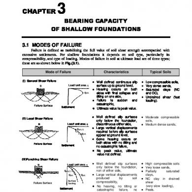
Ch3 Bearing Capacity Of Shallow Foundations (72-164).pdf
February 2021 0
Bearing Capacity Of Shallow Foundations Vesic (1975)
February 2021 0
Bearing Capacity Of Foundations
January 2021 0
Bearing Capacity Of Shallow Foundation
January 2021 0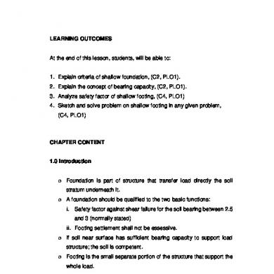
Shallow Foundations
January 2021 0
Bearing Capacity
February 2021 0More Documents from "hact72"

H Bab 6 Ebp
January 2021 1
Ch3 Bearing Capacity Of Shallow Foundations (72-164).pdf
February 2021 0
Ch2 Subsoil Exploration (15-71)
February 2021 2
Askep Ketidakefektifan Bersihan Jalan Napas.docx
January 2021 0
Mola Hidatidosa
February 2021 1