Cheat Sheet Of The Gods
This document was uploaded by user and they confirmed that they have the permission to share it. If you are author or own the copyright of this book, please report to us by using this DMCA report form. Report DMCA
Overview
Download & View Cheat Sheet Of The Gods as PDF for free.
More details
- Words: 4,883
- Pages: 2
Loading documents preview...
Week 2: Soil Types & Phase Relationships
3.1
1.1 Soil: Soil is the accumulation of sediments and mineral particles, typically non-homogenous but not always, influenced by change in moisture content. Differentiated mainly by grain size. Shape/size increase hydraulic and mechanic soil parameters. 1.2 General Definitions: Residual Soil: weathered soil, remaining at original place Alluvial: transported by water Glacial: Transported by glaciers Loess: transported by wind … LOOSE! Marine: deposited in salt/brackish water Expansive: large volume changes with addition of moisture Dispersive: loss of cohesion in water Granular: No cohesion REV: Representative Elementary Volume. The sample size which has a size big enough to represent the sample accurately, can’t be too small, the bigger the sample size the better without getting ridiculous. 1.3 Fine Grained Soils Occurs due to weathering of parent rock(mineral), resulting in formation of groups of crystalline particles at colloidal size(what does that even mean?) High specific surface area(high surface area to mass ratio) Surfaces of clay minerals carry residual negative charges, meaning they aren’t attracted to other shit and can be more dense Attraction between clay particles happens because of van der waals Increasing ion concentration leads to net repulsion Net repulsion = face to face orientation, meaning more dense Net Attraction = face to edge/edge to edge, meaning less close and less dense Absorbed water is held around clay around clay by hydrogen bonding & hydration of cations(CT shiz) 1.4 Equations 𝑉𝑣 Void Ratio[-] Effective Unit 𝛾′ 𝑒= = 𝛾𝑇 − 𝛾𝑤 Weight 𝑉𝑠 [kn/m^3] 𝑊𝑠 𝑉 Porosity[-] Dry Unit 𝑣 𝛾𝐷 = 𝑛= 𝑉𝑇 Weight[kn/m^3] 𝑉𝑡 𝛾𝑇 𝑒 = 1+𝑤 = 𝐺 1+𝑒 = ∙𝛾 1+𝑒
Moisture Content[%]
Degree of Saturation[%]
Total Unit Weight[kn/m^3] 𝛾𝑤 = 𝑒𝑓𝑓𝑒𝑐𝑡𝑖𝑣𝑒 𝑤𝑒𝑖𝑔ℎ𝑡 𝑜𝑓 𝑤𝑎𝑡𝑒𝑟
= 9.81(10)kn/m^3
𝑤 𝑊𝑤 = 𝑊𝑠 ∙ 100% 𝑉𝑤 𝑆= 𝑉𝐴 + 𝑉𝑤 𝑊𝑇 𝛾= 𝑉𝑇 1+𝑤 = ∙𝐺 1+𝑒 ∙ 𝛾𝑤
Unit Weight of Solids [kn/m^3]
Specific Gravity [kn/m^3]
Saturated Unit Weight [kn/m^3]
𝛾𝑠 =
𝑤
𝑊𝑠 𝑉𝑠
𝐺 =
𝑊𝑠 𝑉𝑠 ∙ 𝛾𝑠
&𝐺
∙𝑤=𝑆∙𝑒 𝛾𝑠𝑎𝑡 (1 + 𝑒)𝐺 = 1+𝑒 ∙ 𝐺 ∙ 𝛾𝑤
Week 3: Soil Characterisation & Soil States 2.1 Soil Tests: Moisture Tests: Oven Drying: soil sample taken & measured, then oven dried, measure again. MD = MCDS – MC Mw = MCMS – MCDS w = (Mw/MD)x100% Sieving: chuck soil in sieves, shake for a while, measure each different sized soil, graph on a PSD Analysis→ Uniformity Coefficient: Cu = D60/D10 Curvature Coefficient: (D30)2/(D10 + DD60) Hydrometer Method: wet dirt, put in tube of water, wait for it to settle, observe the layers of different soils, and take continual readings at different time intervals. Some 4 fucked up useless equation, too hard to type! 2.2 Atterberg Limits Liquid Limit: LL→ the minimum moisture content at which soil flows Plastic Limit: PL→ the minimum moisture content at which soil deforms plastically Shrinkage Limit: SL → the moisture content at which soil reduces volume 2.2.1 Limit Indices Plastic Index: PI → IP = LL – PL Liquid Index: LI → IL = [w-PL]/IP Consistency Index: CI → Ic = [LL – w]/IP Activity: A = IP/[% clay by mass] <1 = low activity 1-2 = intermediate activity >4 = high activity 2.2.2 Atterberg Limit Tests Determine LL - Penetration: drop a machine pin into sample, measure penetration, analyse on log log graph. Determine SL – Shrinkage: fill sample and measure, then dry sample and measure again, some dumb equation 𝑚 −𝑚 𝑉 −𝑉 𝛾 𝑆𝐿 = [ 1 2 − 1 2 ∙ 𝑤] I have no idea if this is actually relevant 𝑚2
𝑚2
𝑔
Determine LL – Casagrande Method: mix soil & water in dish, use a U shaped knife and spread/split the soil. Measure gap and see if it reforms, count blows till reforms. Determine PL – Ellipsoidal(Standard): mix dirt and water, roll into a ball and then roll onto the bench into a sausage like thing sort of like play doh until it breaks, simple enough, stupid inaccurate test. NOTE: PSD & Atterberg Limits are used to determine other properties; erosion, penetration(grouting), hydraulic conductivity, workability and more. Week 4: Soil Classification & Compaction
Undefined Soil Classification: G – Gravel S – Sand C – Clay
M – Silt O – Organic Soil P – Peat W – Well Graded P – Poor Graded L – Low Plasticity H – High Plasticity Flow charts are used to sort samples of soil into certain categories, the following is an example, not sure if we need to know how to do this? These classifications are related engineering parameters; strength, compressibility, hydraulic conductivity, workability Applied to dams & roads 1 = highly desirable, like me, 14 = highly undesirable, like you! This is an internationally accepted classification system. 3.2 Compaction Increased density due to compaction leads to; 1. Increased shear strength 2. Reduced compressibility 3. Decreased porosity 4. Resistance to shrinkage Compaction depends on soil types, size of crumbs and many other factors Proctor Compaction Test: the most standard test for compaction I think. Mix soil & water put in mould, “pulverize” it(ram with hammer), weigh sample as well as mould. Then take out of mould, weigh it and determine the moisture content using drying can. 𝛾 𝛾 1 𝛾 Analysis: 𝛾𝐷 = 𝑇 𝑤𝑠𝑎𝑡 = ( 𝑤 − ) ∙ 𝑆 𝛾𝐷 = 1 𝑤𝑤𝑠𝑎𝑡 1+𝑤
𝛾𝑑
𝐺
+
𝐺
𝑆
Plot dry unit weight on y-axis and moisture content on x-axis Draw a smooth connecting curve Also draw a curve for complete saturation 2 tests; standard compaction & modified compaction(4x larger forces for ramming) 3.2.1 Direct Density Measurement Methods Direct Sampling: place hollow cone over soil, use hammer and ram into ground, remove sample from cone, done! 𝑀 𝜌𝑛𝑎𝑡 𝜌𝑛𝑎𝑡 = (bulk density) 𝜌𝑑,𝑛𝑎𝑡 = (dry density) 𝑉
1+ 𝑤𝑛𝑎𝑡
Substitute Method: Method: Fill jar with sand & determine weight of sand-cone apparatus(W1) Determine weight of sand to fill hole (W2) Dig hole, determine weight of excavation (W3) and moisture content, w. After filling hole with sand determine the weight of the remaining sand and apparatus (W4) 𝑊 Dry Unit Weight: 𝛾𝐷 = 𝑉𝑑 Weight of sand to fill hole: Ws = W1 – (W2+W4) Volume of hole: V = W3/𝛾𝐷 Weight of Dry Soil: Wd = W3/(1+w) Balloon Test: Method: Fill cylinder with water, record volume (V1) Excavate small hole, determine weight(W) & moisture content(w) Use pump to invert balloon in order to fill hole Record volume of remaining water in cylinder(V2) 𝑊 Bulk Unit Weight: 𝛾 = Dry Unit 𝑉1 − 𝑉2
𝛾
Weight: 𝛾𝐷 = 1+𝑤 3.2.2 Indirect Density Measurement Methods Standard Penetration Test: drive standard “split”/”spoon” into sample, count number of blows, N, for specific penetration depth. Cone Penetration Test: using standardiesed cone, measure the required thrust to drive the cone into a sampe at a constant rate(10-20mm/second) 𝑒 −𝑒 𝐷𝑟 = 𝑒 𝑚𝑎𝑥 = WTF! −𝑒 𝑚𝑎𝑥
𝑚𝑖𝑛
Plate Load Test: there is a hydrulic pump measurign force(force metre) as a plate is loaded, measuring the hardness of the ground, I think maybe some penetration will occur? 3.3 Dispersion Chemically supported erosion process Dispersive clays, disperse in water & are erodible under rainfall Dispersive soils are common in QLD To test dispersion: Place soil “crumbs”” in water dish, if the water becomes turbid or cloudy around the crumb, then it is dispersive, common sense, fuck! Week 5: Darcy’s Law & Hydraulic Conductivity 4.1 Hydraulic Head/Potential: Hydrostatic pore water pressure, uw, increases with depth below the water table uw = 𝛾𝑤 ∙ 𝑧𝑤 where zw = depth below water table negative pore water pressure occurs above the water table causes deformations of soil during shrinkage Potential Concept: {B} 𝑢𝑤 𝑣2 𝐻=𝑍+ + 𝛾𝑤 2𝑔 H = total head(m) Z = elevation head(m) v = velocity(m/s) 𝑣2 5 = velocity head(m) 2𝑔 For laminar flow;
𝑣2 2𝑔
=0
Hydraulic Head: ℎ =𝑍+
𝑢𝑤 𝛾𝑤
[m]
Hydraulic head is a specific measurement of liquid pressure above a datum Velocity head is due to the bulk motion(kinetic energy) Elevation Head is due to the fluids weight, the gravitational force acting on a column of fluid 4.2 Darcy’s Law Saturated Seepage for laminar flow, seepage is the slow escape of a liquid or gas passing through a porous material. Q = -k ∙ i ∙ A Q, Discharge is the volumetric flow rate per unit time(m2/s) k, proportionality factor i, hydraulic gradient combines both change in head and length
ℎ2 − ℎ1 𝑖= 𝐿 Hydraulic head is a gradient against 2 or more hydraulic head measurements A, cross sectional area (m2) q, specific discharge(Q/A) [m/s] Filter Velocity: apparent velocity of water through soils 𝑄 Δℎ 𝑑ℎ 𝑣𝑓 = = −𝑘 = −𝑘 𝐴 Δ𝑠 𝑑𝑠 Pore Velocity: real velocity of water through pores 𝑣𝑓 𝑣𝑝 = , n = porosity, for fine grained soils use effective porosity ne 𝑛 Hydraulic head(as a combination of pressure head and geodetic height) causes water to flow(most important concept in groundwater hydraulics) 4.3 Hydraulic Conductivity This is a soil property that describes the ease at which water can move through pore spaces, but for dumb people like me it means how easily water can travel through soil. It ca be calculated heaps of different ways using multiple different tests and formulae Typical values: 10-3 to 10-8 [m/s] Constant Head Test: pretty much, just fill up a container with sand/soil, connect funnel ad outlet, let water flow through mechanism and measure discharge do it twice or more with different heads(place the funnel higher or lower and measure discharge for both 𝑄𝑖 𝐿 k𝑖 = × 𝐴 Δℎ𝑖 𝜂 Normalize Result: 𝑘20 = 𝑘𝑡 × 𝑡 𝜂20
Falling Head Test: 𝑎×𝐿 ℎ 𝑘𝑡 = × ln( 1) 𝐴×Δ𝑡
ℎ2
Kt is the hydraulic conductivity for temperature, T. a = area of pipe(m2) A = area of sample(m2) L = length of sample(m) h1 = hydraulic head at beginning and h2 = hydraulic head at end Note: when testing for k. Use de-aired water Use full saturation Use homogenous structure, if not segregation occurs and that fucks up results Consider temperature Conductivity of filter stones must always be greater than of the sample Factors influencing conductivity Fluid: Viscosity, density, unit weight of water Soil: Porosity, mean pore diameter, tortuosity(how pores are connected to each other, “connectivity”) Conductivity from PSD Empirical method of Hazen(for soils with Cu<5, 10⁰C) k = 0.01∙d02 [d0 = mm] method of Beyer (gravel and sand, 0.06
Horizontal flow: 𝑘ℎ = ∑
𝑙𝑖
=
⁄𝑘 + ⁄𝑘 +⋯+ ⁄𝑘 1 2 𝑛 𝑙1 ∙𝑘1 + 𝑙2 ∙𝑘2 +⋯+ 𝑙𝑛 ∙𝑘𝑛 𝑙1 +𝑙2 +⋯+ 𝑙𝑛
Variability of k is bigger than any other soil parameter Permeability depends only n the porous medium(fluid does not affect it) where k depends on both soil and fluid 4.4 Permeability This is the ability of a porous material(soil) to transmit water, differing to hydraulic conductivity which is the ease at which fluid travels through a porous medium depending on both fluid and material properties. Week 6: Hydraulic Conductivity & Flow Nets 5.1 Hydraulic Conductivity Again: Field Measurement: 𝑟2 𝑞 [ln (𝑟1 )] 𝑘= ∙ 𝜋 ℎ2 2 − ℎ1 2 Used for wells and pumps and shiz(unconfined flow) Used for coarse grained soils and fractured rock 5.2 Limitations of Darcy’s Law Reynold’s number: this is a dimensionless umber that s a measure of the ratio between inertial forces and viscous forces 𝑅𝑒 =
𝑣𝑓 ∙𝑑𝑒 𝑣
2 ∙𝑇
∙ 3(1−𝑛) (laminar flow)
Vf = filter velocity [m/s] de = effective diameter [m] ρ = density v=kinematic viscosity T=tortuosity Validity of Darcy’s law (Laminar Flow) Hydraulic gradient limit is used for the limit of laminar flow
i = 0.222(1/de3) where de is measured in mm Measurement of post lamina range(between laminar and turbulent), use Forcheimer’s Law i = a∙vf + b∙vf2 a =1/k b=fit parameter, given to you For fine grained soils the hydraulic gradient must overcome a specific yield stress to initiate a flow of water (no flow): q = 0 for 0 < i < i0 (flow): q = kf(i – i0) for i > i0 (darcy) Darcy’s law only valid for representing flow if there is a linear relationship between hydraulic gradient and specific discharge(or filter velocity) In the pre-laminar rage there is a “stagnation gradient” i0 that must be overcome to initiate flow In post-laminar range(for coarse grained soils & for i > i limit) the flow starts to become partly turbulent(Re>1) Experiments with partly turbulent flow can be analyzed with Forchiemers law to receive k for laminar flow 5.3 Seepage 5.3.1 1D Seepage 𝛾𝑠𝑎𝑡𝑢𝑟𝑎𝑡𝑒𝑑 − 𝛾𝑤 𝐶𝑐𝑟𝑖𝑡𝑖𝑐𝑎𝑙 = ≅1 𝛾𝑤 For upwards vertical flow in sand 𝜎𝑣′ < 0 5.3.2 2D Seepage 𝑑𝑣 𝑑𝑣 Continuity Equation: 𝑥 + 𝑧 = 0 𝑑𝑥 𝑑𝑧 Assuming homogenous and isotropic conditions, both pore water and soil are incompressible Vx and Vz are both apparent velocities in x and z directions, not actual velocities 𝑑ℎ Darcy’s Law: Vx = kx ∙ 𝑑𝑥 𝑑 2ℎ
𝑑 2ℎ
Laplace Equation: 2 + 2 = 0 𝑑𝑥 𝑑𝑧 In terms of hydraulic head, k = kx = kz, used for flow nets, used for anisotropic conditions(antistrophic = directionally independent) 𝑑 2ℎ
𝑑 2ℎ
Steady State Seepage: 𝑘𝑥 𝑑𝑥 2𝑥 + 𝑘𝑧 𝑑𝑧 2𝑧 = 0 hx ad hz are heads in each direction 5.4 Flow Nets Flow nets are used to map confined flow through horizontal layers Assume: stationary conditions(Qin = Qout), homogenous, isotropic Total potential difference is linearly reduced along the sample (∆Ltot) ∆htot = hu – hd i = ∆htot/∆Ltot ∆htot is divided into N equal potential drops along the flow net and are known as equipotential lines(vertical lines) All lines must be 90⁰ at top and bottom of diagram Flow lines are used to form a quadratic flow net, M, flow tubes(horizontal lines) Normally not a natural number, eg. 2.3 In each flow tube the same Q will flow Total discharge: Q = k∙i∙A = k(∆htot/∆Ltot)∙b Q = M∙∆Q = (M/N)∙k∙∆htot Specific discharge, q: discharge in a single flow tube) ∆Q = k ∙i local ∙ A = k∙∆hi /(∆L ∙ ∆b) (∆L ∙ ∆b) = 1 & ∆hi = ∆htot/N therefore ∆Q = k ∙∆hi = k∙(∆htot/N) Volume dependent Seepage Force: S = ilocal ∙γc ilocal = ∆hi/∆L Total Seepage Force: S = s∙V V = volume of soil affected by flow of water Rules for flow nets: Sets of flow line and equipotential lines are drawn within a seepage zone to form a flow net A permeable boundary is an equipotential line(max or min) [vertical] An impermeable boundary is a flow line [horizontal] Phreatic surface = surface exposed to atmosphere Right angles must be made with top line(phreatic surface) and bottom but not necessarily middle lines(but sort of close to 90⁰, they need to make rough squares at the intersections of flow tubes ad equipotential lines) Week 7: Flow Nets 6.1 Errors in Flow Net Construction Usual errors in flow nets are sue to: Extraneous equipotential lines Disapperaing flow lines, not connected the whole time Disappear through the bottom Flow lines and equipotential lines not intersecting at 90⁰ Digram is a correct flow net 6.2 Constrcution 6.2.1 Confined Flow Define boundary conditions(max and min equipotential lines, shortest and largest flow lines) First estimate of starting and ending points of flow lies ad equipotential lines First sketch of lines and readjustment of starting and ending points, adjust for 90⁰ squares Proportions of flow net can be subdivided with square lines to even up the net 6.2.2 Unconfined Flow Definition of boundary conditions, guess location of phreatic surface First estimates of start and end points for equipotential and flow lines First sketch, with readjustment Improve by drawing circles within each intersecting square This is pretty much guess work and an arts degree combined, good luck! Several types of flow nets: Embankment with chimney, homogenous, rock toe drain and flow through dams 6.3 Analysis Flow through seepage zone: q = k∙∆∙(M/N)
Filter velocity, vf varies through seepage zone, the “apparent” velocity increases as dimensions decrease, like a nozzle. Pore water pressure, uw, from the side with the highest total head to the side with the smallest, via each equipotential lines(even drops in pressure per equipotential line) Flow nets with different k values: Flow lines are refracted (width/shape changes) on the crossing interface between k values (W1/k1) = (W2/k2) W = width of flow tube For anisotropic soils shit just gets dumb Flow nets may be used with a transformed scale Don’t really know what this means? 𝑘
Reduction of horizontal length: 𝑥 ′ = √𝑘 𝑧 ∙ 𝑥 𝑥
𝑀
Discharge: 𝑞 = ∆ℎ ∙ 𝑁 ∙ √𝑘𝑧 𝑘𝑥 6.4 Special Cases Local effects of seepage stresses Quick conditions can occur if σ’v < 0 where: σ’v = effective stress Can be avoided by decreasing i Increasing L using a cutoff and/or decrease h by dewatering and/or increase σ’v by surcharging Surcharging = extra loading above soil line being supported by a retaining wall Seepage stresses can cause heave in clays, in extreme cases can cause piping Piping is the erosion of soil leading to sink holes, sort of creates natural pipes in the ground. In granular soils, seepage stresses lead to erosion 6.5 Overview 2D seepage can’t be described with a flow net Unconfined slow = top surface is exposed to atmosphere(phreatic surface) pretty much means it is not confined Flow nets provide info on uw and hydraulic forces which have to be taken into account for safety of hydraulically loaded structures Increased hydraulic gradient leads to local erosion processes >40% dysfunctions/failures in embankments due to erosion Week 8: Soil Stress & Principle Effective Stress 7.1 Force Pressure & Stress Pressure & Stress are dependent on Area Pressure & stress vary with space Multiple components of stress, x, y & z Internal pressure(P) = External Force(F)/Area(A) Pressure ad stresses are better related to the material mechanical changes(damage, failure, stretching, …) rather than forces 9 7.2 Effective Stress Effective Stress Principle: σ’ = σ - uw σ = total stress, the weight of everything above a certain point, including water, uw is the pre water pressure. Used for saturates soils in dry soils σ’ = 0 change in σ leads to deformations and changes in strength the soil grains and pore water are assumed to be incompressible in a saturated soil, deformation on the application of stress is directly related to the expansion of water, which means its related to k, hydraulic conductivity Sand Shear Strength (τ): proportional to σ’, τ = tanφ ∙ σ’ where; φ = internal angle of friction Clay shear strength(τ): τ = cu or c’ Also proportional to σ’, but the constant of proportionality is dependent o the “overconsolidation ratio” (OCR) (σ/ τ)NC = constant [typically = 0.25] NC = normally consolidated, OC = over consolidated m = a value experimentally found, equal to 0.8 𝜏 𝜏 ( )𝑂𝐶 = ( )𝑁𝐶 ∙ (𝑂𝐶𝑅)𝑚 10 𝜎′ 𝜎′ Drained Behavior: In high permeability soils(sand ad gravel) any excess pressure gained by an applied stress generally dissipates instantaneously, the applied stress transferring instantly to the soil skeleton pretty much means a drained situation has no real difference quick conditions or “liquefaction” are an exception, the rate of stress application is faster than drainage rate and the seepage stresses exceed the strength of the soil(pure water strength over rules) Short Term Undrained: pretty much the same as long term drained, it means in saturated soils of low permeability any excess stress is taken as excess pressure and applied to the soil skeleton. (In a question add the extra pressure) Loss of effective stresses can be caused by hydraulic forces Critical hydraulic gradient Seismic excitation(I think this means small vibrations in soil due to increased pressure) When liquefaction and earthquakes combine, buildings die. 7.3 Geostatic Stress This stuff is pretty much quiz 3. σv = total vertical stress, this is equal to the weight of everything above this point uw = hydrostatic pore water pressure, increases with depth under ground effective vertical stress(σv’), this is the difference between total vertical stress and pore water pressure σv’ = σv –uw σH’ = k0 - σv’ Total vertical stress sue to wet soil is equal to unit weight multiplied by depth at that point σv = 𝛾𝑇 ∙ z Week 9: Stress & Strain/Mohr Circle 8.1 General Consideration Engineers use a rational approach to design considering continuum mechanics & differential equations to represent structural conditions leading to an initial boundary value problem (IBVP) IVBP’s are solved to asses safety of failure(collapse), safety of large deformations(serviceability) and safety of other problems such as water leakage
Assessing the following: Seepage: need understanding of hydraulic conductivity and water flow Slip lines: understanding of strength Settlement: understanding of deformation due to loads & deformations in time due to pore water movement (consolidation) To solve IVBP’s all materials must be characterized in lab tests(morphologically, mechanically, hydraulically) Pretty much IVBP’s are tests to represent conditions of future designs for big ass structures 8.2 Representations of Stress Conditions Stress state in soil is described by normal and shear stresses applied to the boundaries of the sample Stress states can be plotted 2 ways Pair of coordinates (σz’ , τxy) and (σx’ , -τxy) Mohr’s circle of the effective principle stresses (σ1 and σ3) 8.3 Mohr’s Circle At an angle of 2θ to the horizontal of the circle is a representation of the stress condition o a plane at an angle of θ to the direction of the minor principle stress, σ3 The circle represents the stress states on all possible planes within the soil element All info is then represented on a failure envelope A stress condition represented by a point above the failure envelope is not possible(failure occurs with small shear stress) Relationships between shear strength parameters & effective principle stress at failure can be found from shear stress (τf) and normal stress (σf) acting in the failure plane. τf = 0.5(σ1’ – σ3’)sin(2θ) σf’ = 0.5(σ1’ + σ3’) + 0.5(σ1’ – σ3’)cos(2θ) where: θ = the theoretical angle between minor principle stress(σ3’) and the failure plane, hence why 2θ = 90⁰ + φ’ and θ = 45⁰ + (φ’/2) Mohr-Coulomb Criterion: this defines the relationship between principle stresses at 11 failure and material parameters, φ’ and C’ (σ1’ – σ3’) = (σ1’ + σ3’)sin(φ’) + 2C’cos(φ’) (σ1’) = σ3’tan2(45⁰ + [φ’/2]) + 2C’tan(45⁰ + [φ’/2]) For a given state of stress it is apparent that because of (σ’ = σ – uw) that the Mohr circle will have to shift when dealing with effective stresses, the same diameter will be used it will just be moved 8.4 Overview Tests with soil(mechanical and hydraulic) are needed to quantify material parameters in order to calculate safety against failure, settlements , … Mohr’s circle is used to describe stress states of soil both before and after failure Stress and strain invariants are used to show evolution of stresses for changing stress conditions or deformations(stress paths) Week 11: Mechanical Behaviours 9.1 Mechanical Behaviours Modes of failure in triaxial compression Shear plane failure(brittle) Barrelling(plastic failure) Combination of both(intermediate failure) Elastic behavior(idealized) has deformation that is recovered after loading Behavior can be linear or non linear Can act both elastically or brittle(rigid) Elasto-plastic(idealized) behavior: deformation is permanent after unloading Behavior can be linear or non linear Can act elastically or brittle Can act with hardening or softening Loose “normal” porous soils act in a ductile(plastic) manner Dense compacted/consolidated materials act in a brittle way(sudden loss of strength) In “realistic” soils there is always some deformation necessary to actuate friction Week 12: Soil Strength
C’ = effective cohesion Failure due to wall movements
φ = friction angle
Changes in stress conditions is represented by sets of Mohr’s circles This page from lectures pretty much sums up Mohr and his fucking annoying circle!
Week 13: Soil Testing and consolidation
Rope Bullshit Test
Week 12: Soil Testing 11.1 Direct Shear Test Shear Box Test: relatively quick and simple, soil is forced to shear at the interface between the two halves of the box during shearing, the shear stress and normal stresses are measured the effect of large shear displacement is obtained by reversing the shear box after initial displacements are measured then repeating a bunch of times to achieve a steady(residual) shear strength Ring Shear Test: pretty sure a sample of soil is just twisted until it fails Effective parameters = C’ & φ’ Effective residual parameters = Cr & φr Advantages of this test = this test can also be used for measuring angle of friction developed at an interface of soil and other material Disadvantage = major assumption that stresses within sample are uniformly disturbed 11.2 Conventional Triaxial Test Conventional triaxial test carried out in 2 stages 1. Isotropic compression → consolidation(in time) or not τ ≈ 0 Consolidated(C) or unconsolidated(U) 2. Loading(shearing) to failure with drainage or not τ > 0 Drained(D) or undrained(U) An unconsolidated and drained test is highly uncommon 11.3 Unconfined Compression Test This is a special case of a triaxial test, determining Unconfined compression strength (UCS) Special case: σr = o, therefore dimensionless Only 1 stage, loading until failure(quick test) Samples are capable of being formed as self-supporting cylinders Ultimate Strength
10.1 Mechanical Behaviours Soil moduli is also known as the soil stiffness, it can be determines from stress-strain relationships
10.2 So far … We have been learning about strength for ages pretty much, this is just a bit of a recap of the important bits Total stress increases, σ with depth Pore water pressure, uw, reduces the total stress to effective stress, σ’ Normally horizontal stresses < vertical stresses Stress states/conditions (both 2D and 3D) can be visualized using Mohr’s circle Difference in stresses at different locations leads to shear stresses τ When shear stresses exceed shear strength, τf failure occurs Therefore there is a maximum limit of shear strength soil can withstand The maximum shear strength is dependent on the normal stresses σn acting in the shear plane A failure envelope is found by a combination of points of maximum shear stresses and normal stresses A linear relationship known as the mohr-coloumb criterion maps shear and normal stresses at failure τf = C’ + σf tan(φ’)
11.6 Consolidation Drained Test (CD) 2 stages, consolidation and loading to failure with drainage During consolidation, volume change with respect to isotropic pressure can be determined Pore water pressures are zero, total stresses = effective stresses Only drained parameters can be found 11.7 Overview Mohr’s circle contains NO info about deformations Shear parameters and stress strain relationships are dependent on density During consolidation(phase 1) load deflection curves are measured which can be used to asses consolidation parameters Residual parameters are measured by repeating the shear box test Triaxial tests are differentiated by consolidation and hydraulic conditions(drained/undrained) Drained conditions means pore water pressure changes = 0 Tests must be done very small to eliminate/reduce development of uw Undrained conditions means no change in volume, but uw can change During CU tests effective parameters can be determined
Coefficients of Primary Consolidation Compression Index (𝑪𝑪 ): Gradient between initial state of normally consolidated clay and final stress condition for prediction of settlements Recompression (𝑪𝒓 )/Expansion (𝑪𝒆 ) Index: Gradient between initial state of over consolidated clay and initial state of normally consolidated clay Coefficient of Volume Compressibility (𝒎𝒗 ): Relates the vertical stress with the vertical strain by the following rate equation:
Oedometer Test Test procedure for primary consolidation Each dead weight is added and left for a period of time. During this time the vertical displacement ∆𝑢𝑧 is measured For each increment of time, a pair (∆𝑢𝑧 , 𝜎𝑧′ ) is obtained Summary
Useless shit I could fit in.
11.4 Unconsolidated Undrained Test (UU) Only 1 stage, loading until failure Drainage is prevented Repeat test with multiple samples extracted from the same depth and position to give an average(line of best fit for horizontal line Su) Mean pressure does not affect strength because the confining pressure only affects the pore water pressure Disadvantages: unconfined strength is not intrinsic of material, varies from one point to another in the same soil mass, varies with depth However C’ and φ’ the material parameters do not vary greatly with depth
11.5 Consolidated Undrained Test (CU) 2 stages, consolidation and loading to failure without drainage During consolidation the volume change with respect to isotropic pressure can be determined During loading there is no volume change cause valves are closed If pore water pressure changes are measured, effective parameters can also be calibrated
Related Documents

Cheat Sheet Of The Gods
February 2021 0
The-sense-of-rhythm-cheat-sheet-1
February 2021 0
Scrum Cheat Sheet
January 2021 1
Agile Scrum Cheat Sheet
February 2021 0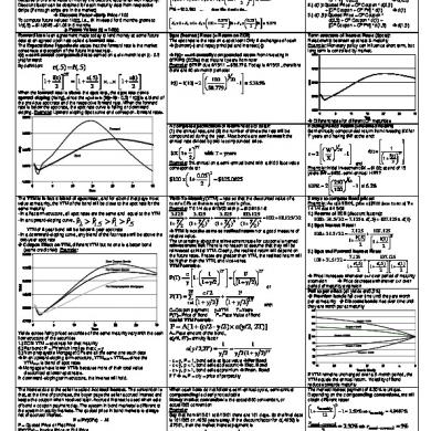
Bonds Exam Cheat Sheet
February 2021 1
Neo Harmonics Cheat Sheet
January 2021 1More Documents from "Cendron Omar"
Cheat Sheet Of The Gods
February 2021 0
Anatomy Of A Hostage Rescue - Ada427693
January 2021 2
Manual De Acupunctura
February 2021 3
Esquema Opo.pdf
January 2021 1
