Finance Cheat Sheet (1)
This document was uploaded by user and they confirmed that they have the permission to share it. If you are author or own the copyright of this book, please report to us by using this DMCA report form. Report DMCA
Overview
Download & View Finance Cheat Sheet (1) as PDF for free.
More details
- Words: 2,350
- Pages: 2
Loading documents preview...
Capital Budgeting – process of planning & managing firm’s investment in long-term assets Capital Structure – mix of debt & equity maintained by firm Working Capital – planning & managing firm’s current assets & liabilities Agency Problem – possibility of conflicts of interest between shareholders & management of firm Corporate Governance – rules for corporate organization & conduct Money Markets – financial markets where short-term debt securities are bought & sold Capital Markets – financial markets where long-term debt & equity securities are bought & sold Financial Engineering – creation of new securities or financial processes Derivative Securities – options, futures, other securities whose value derives from price of another asset Regulatory Dialectic – pressures financial institutions & regulatory bodies exert on each other Non-cash Items – expenses charged against revenues that do not directly affect cash flow (ex. depreciation) CFFA – total of CF to bondholders/shareholders: OCF, Capital Spending, NWC (aka free cash flow) OCF – cash generated from normal business activities Dividend Tax Credit – reduced effective tax rate on dividends Capital Gains – increase in value of investment over its purchase price OR Loss Carry-forward, – using year’s capital CFFA Carry-back Interest paid on LT debt losses in past/future years EBIT to offset capital gains + NI + Depreciation - Change in LT debt - Taxes - Change in total equity = Operating Cash Flow = CFFA Ending Fixed Assets OR - Beginning Fixed Assets Interest paid on LT debt + Depreciation - Net cash from financing = Net Capital Spending = CFFA Ending NWC % of Sales Method - Beginning NWC 1. everything on IS by g = Change in NWC 2. ST A & L (not N/P) by g Operating Cash Flow 3. g’=(1+g)(x) x = - Net Capital Spending %capacity - Change in NWC a) if g’ < 1, FA stay at = CFFA current value b) if g’ > 1, multiply FA by amount
Common-size Statement – presents items in % FV – amount investment is worth after 1 or more periods Common-base-year Statement – presents items relative to base (compound value) year Compounding – accumulating interest in invest. over time to Financial Ratios – relationships from financial info used for earn more int. comparison Interest on Interest – earned on reinvestment of previous Liquidity Ratios – ability to meet short-term obligations without interest payments undue stress Compound Interest – earned on initial principals & int. Quick Ratio – ST liquidity after removing inventory reinvest. prior periods Cash Ratio – ability to pay off current liabilities with cash Simple on original FV = PVInterest x (1+r)T – earnedCash Flows principal amount Annuity: Interval Measure – how many days or operating expenses can Payment = PV = FV/(1+r)T PV = (C/r) x 1 – [1/ current assets cover (1+r)T] annuity end (ordinary) Financial Leverage Ratios – LT ability to meet obligations FV = C/r x (1+r)T – 1 Payment = Equity Multiplier – dollar worth of assets each equity $ has claim annuity bgn (due) to Mortgage: PV = C/r Leverage Ratios LT Debt Ratio - %Financial of total firm capitalization funded by long-term perpetuity C/Y = 2 Annuity – level stream of cash flows for fixed period of time Total Debt Ratio = (TA – TE)/TA **<.5 debt Annuity Due – cash flows occur at beginning of period Debt/Equity Ratio = TD/TE = EM – 1 **<1 Perpetuity – annuity in which cash flows continue forever Consol – Equity Multiplier = TA/TE = TD + (TE/TD) = TD/TE + 1 = type of perpetuity DE Ratio + 1 **<2 Growing Perpetuity – constant stream of cash flow without end LT Debt Ratio = LT Debt/(LT Debt + TE) Du Pont Growing Annuity – finite # of growing annual cash flows Times Interest Earned = EBIT/Interest Identity Stated/Quoted Interest Rate – expressed in terms of interest Cash Coverage Ratio = (EBIT + Depr)/Int ROE = NI/TE payment made each period Liquidity Ratios Profitability = (NI/Sales) Effective (EAR) –t]/r} interest rateAnnuity expressed if it were Annuity Annual PV = C xRate {[1-1/(1+r) FVas Factor = Current Ratio = CA/CL **>1 Ratios or >2 (Sales/TA) ((1+r)t – 1)/r Quick Ratio = (CA – Inv)/CLPM **>1 = NI/Sales (TA/TE) = Cash Flow = PV x r Annuity PV Factor = Cash Ratio = Cash/CL ROA = NI/TA (PM)(TAT) (1/r) x (1-PV Factor) NWC = NWC/TA ROE = NI/TE Coupon – stated interest payment Market Value PV of Growing Perpetuity = C/(r-g)made on PVbond of Growing Annuity = Interval Measure = CA/Avg Daily Face/Par Value – principal amount of bond repaid at end of term Ratios Op Costs Coupon Rate – annual coupon divided by face value of bond Price-Earnings Ratio = Asset Turnover Ratios Share $/EPS Maturity Date – date when principal amount of bond is paid Inventory Turnover = COGS/Inv Market-to-book Ratio = Yield to Maturity (YTM) – market interest rate that equates bond’s Days’ Sales in Inv = 365/Inv PV of interest payments & principal repayments with its price MVPS/BVPS Turnover EV/EBITDA = [MV of Equity +Indenture – written agreement between corp. & lender detailing Net Invest in FA = (NFA – END Days’ Sales in Rec = 365/Rec terms of debt NFABEG) + Depr Turnover Debenture – unsecured debt, maturity of 10+ years Note – TD = CL + LTD Receivables Turnover = Sales/A/R maturity -10 years BVPS = TE/Shares Days’ Sales in Pay = 365/Pay Sinking Fund – account managed by bond trustee for early bond SPS = Sales/Shares Turnover redemption Price-Sales Ratio = Share $/SPS Pay Turnover = COGS/A/P Call Provision – option to repurchase bond at specified price before EPS = NI/Shares NWC Turnover = Sales/NWC maturity FA Turnover = Sales/Net FA Planning Horizon – long-range time period financial planning Call Premium – amount by which call exceeds par value of bond Deferred Call – call provision prohibiting company from redeeming processes focuses on bond early Aggregation – small invest. proposals of each operational unit are Call Protected – bond during period in which cannot be redeemed added, treated as 1 project % of Sales Approach – accounts are projected depending on by issuer Canada Plus Call – compensates bond investors for interest predicted sales level Plug Variable – adjusted to make sure pro forma balance sheet differential Retractable Bond – may be sold back to issuer before maturity balances Clean Price – price of bond net of accrued (quoted) External Financing Needed (EFN) – amount of financing to Total Dollar Return = Dividend Incomeinterest + Capital Gain (loss) CF to Creditors = interest paid – net new LTD Dirty Price>–coupon price of rate, bond including accrued int., buyer pays If YTM bond price < par balance both sides of BS = Increase in Price + Coupon Payment CF to Shareholders = dividends paid – net new equity Dividend Payout Ratio = Cash Div/NI Div = NI – Change in(full/invoice price) value (DISCOUNT) Total Cash if Stock is Sold = Initial Investment + Total Return CFFA – CF to Creditors + CF to Shareholders E Plug Variable If YTM < coupon Dividend Yield = rate, Dt/Pt par value < bond NI = dividends + addition to retained Retention/Plowback Ratio = RE/NI Div = Payout Ratio x price (PREMIUM) t Capital Gains Yield = (Ptt+1 t)/Pt Bond Value = C x (1-1/(1+r) )/r –+PF/(1+r) Current Yield = Earnings OR EBT – EBT x tax rate New NI Fixed PR % Total Return = Dividend Yield + Capital Gains Yield Net Capital Spending = FA bought – FA sold Full Capacity Sales = Current Sales/Capacity % of FA = CPN/PRC = (Pt+1 + Dt)/Pt price = 100 F4: Bond Calculation *quoted Cap. Gains Net Acquisitions = total installed cost of capital FA/Full Capacity Sales Var(R) = (1/(T-1)) x [(R Yield = YTM – Cur. Yield 1R )2+…+(RT- R )2] *use sx for acquisitions – adjusted cost of disposals Max Sales Growth = (Full Capacity Sales/Current Sales) – 1 d1 = current date PRC = clean price Fisher standard deviation Terminal Loss = UCC – adjusted cost ofcurrent disposals Common Shares TA – L –– difference RE Incremental Cash=Flows b/w firm’s future CFs with Dividend Growth Model – determines price of Effect = 1+R =Average (1+r)(1+h) Recaptured CCA – adjusted cost of disposal – UCC Internal Arithmetic = Sum of Returns/# of Returns = x project & Growth without Rate = (ROA x R)/([1-[ROA x R]) stock maturity date YLD = YTM OR R AverageGains Tax Rate taxable income Sustainable Growth Rate = (ROE xbased R)/([1-[ROE x R]) **AKA Stand-Alone Principle – evaluation on incremental CFs d2 = Capital Yield=–total rate taxes/total at which value of investment under F1:1VAR max % sales increase 1/T Sunk Cost – incurred & cannot be removed, should not be grows Geometric Average = [(1+R1) x (1+R2) x…x (1+RT)] – 1 Common Stock – equity without priority for dividends or considered Nominal Return = Total $ Return/Original Price Opportunity Cost – most valuable alternative given up in bankruptcy *use Fisher equation for real return & risk-free rate (R =
Constant Dividend Growth OCF PO = D1/(r-g) = DO x (1+g)/(rBasic Approach = EBIT+D-Taxes g) Top-Down Approach = Sales-Costs-Taxes *will be paid *Just been Bottom-Up Approach = NI+D Constant paid Tax Shield Approach = (S-C) x (1-TC) + (D x TC) Dividend F2: Compound Interest PO = D/r n=99999 I%=(r-g)/(1+g) PV Tax Shield on CCA = ([IdTc]/d+k) x ([1+0.5k]/1+k) PV F2: Compound PMT=D1/(1+g) OR [DO x – ([SndTC]/d+k) x (1/[1+k]n) Salvage Interest (1+g)]/(1+g) Value Expected Return – return on risky asset expected in future n=99999 Expected Divided: DT = DO x Remaining Tax Shield = (UCC-S) x d x TCPortfolio /(d+k) – group of assets (ex. stocks & bonds) held by T (1+g) Straight-Line Depreciation = (Initial Cost – Gross Salvage investor Expected Stock Price: PT = PO Value)/Years Portfolio Weights - % of portfolio’s total value in asset x (1+g)T TC corporate tax rateDeclining Balance (CCA) = d x UCC Non-Constant Growth Systematic Risk – influences large # of assets (aka market I total investment capital 1. Compute dividends before constant growth risk) added to pool DT = DO x (1+g)t Unsystematic Risk – affects small # of assets (unique/assetEXAMPLES TO FIND d CCA rate 2. Find expected FV of stock at time of constant specific risk) NPV: k discount rate growth Principle of Diversification – spreading investment across # Sn salvage value PT = D1 x (1+g)t/(r-g) OR PT = DT/(r-g) of assets eliminates some of risk Mn asset life in years F2: Compound Interest OR Int Rate: Systematic Risk Principle – amount of systematic risk n=99999 I%=(r-g)/(1+g) n=4 present in risky asset relative to average risky asset P/Y=1 P/C=1 Security Market Line (SML) – positively sloped straight line PMT = dividends before growth PV=-1 FV=1+r displaying relationship between expected mean and beta *ex. compounded Market Risk Premium – slope of SML (difference between quarterly expected return on market portfolio and risk-free rate) 3. Compute current PV of stock Capital Asset Pricing Model (CAPM) – equation of SML t PO = (D1 + PT)/(1+r) showing relationship between expected return Rate and beta Risk Premium = Expected Return – Risk-free F3: Cash Flow, I%=r F2: Opportunities Compound Interest Stock Valuation Using OR Growth = E(R) - Rf Multiples EPS = Div Expected Return = E(R ) = jRj x Pj Pt = benchmark PE ratio x Value of share = EPS/r = Div/r Return Variance = 2 = j [(Rj – E(R)]2 x Pj Stock price after project = Portfolio Expected Return = E(Rp) = [x1 x E(R1)] + [x2 x E(R2)] NPV – difference between investment market value and (EPS/r) + NPVGO +…+ [xn x E(Rn)] cost Portfolio Variance = 2p = (x21 x 21) + (w22 x 22) + 2 x w1 x w2 Discounted Cash Flow Valuation (DCF) – valuing x p x 1 x 2 investment by discounting future cash flows Total Return = Expected Return + Unexpected Return Discounted Payback Period –time for investment’s DCFs (Systematic + Unsystematic) to equal initial cost = R = E(R) + U (m + ) Internal Rate of Return (IRR) – discount rate that makes Beta = I = piM x (i/M) NPV 0 Beta of Portfolio = p = wj x j NPV Profile – graph of relationship between NPVs and discount rates Reward-to-risk Ratio = [E(RA) - Rf]/A (aka slope) Multiple Rates of Return – problem in using IRR CAPM = E(Ri) = rf + i[E(RM) – rf] NPV Payback Period Average Accounting *Find CCATS then input cash Premium flows Risk – excess return required from investment in Arbitrage Pricing Theory (multiple) = rf + 1 x (E(R1) – rf] + F3: Cash Flow F3: Cash Flow Return 2 x (E(R2) – rf] +…+K x (E(RK) – rf] I% = required rate I% = 0% AAR = Avg. NI/Avg. BV risky asset over risk-free environment Variance – average squared deviation between actual return & List 1 = cost, cash List 1 = cost, cash Avg. BV = Cost/2 flows flows *accept if AAR > pre- average return Standard Deviation – positive square root of variance *if NPV > 0, *accept if PBP < Normal Distribution – symmetric, bell-shaped frequency invest pre-set limit Discounted Payback IRR distribution defined by mean & standard deviation Period F3: Cash Flow Value at Risk (VaR) – maximum loss used by banks to F3: Cash Flow I% = required rate manage risk exposures I% = required rate List 1: cost, cash flows Geometric Average Return – average compound return List 1 = cost, cash flows *accept if IRR > earned per year over multi-year period *always lower *accept if pays back on required return Arithmetic Average Return – return earned in average year discounted basis within *If signs change twice, 2 over multi-year period *nominal return Profitability Index Efficient Capital Market – security prices reflect available PI = 1+(NPV/initial investment) = Benefit/Cost Ratio
Common Stock Cash Flows PO = (D1+P1)/(1+r) F3: Cash Flows, I% = r
Related Documents

Finance Cheat Sheet (1)
February 2021 0
Price Action Cheat-sheet(1)
January 2021 4
Scrum Cheat Sheet
January 2021 1
Agile Scrum Cheat Sheet
February 2021 0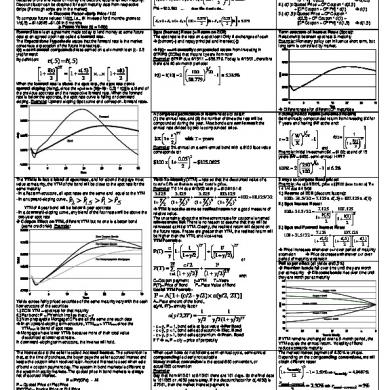
Bonds Exam Cheat Sheet
February 2021 1
Neo Harmonics Cheat Sheet
January 2021 1More Documents from "Cendron Omar"
Finance Cheat Sheet (1)
February 2021 0
Allan Holdsworth-extreme-legato-lessons-allan-holdsworth.pdf
February 2021 0
Composing Interactive Music
February 2021 1
Giordano Bruno Y La Tradicion Hermetica - Frances A. Yates
January 2021 1
